Genomic annotation in Bioconductor: The general situation
Basic annotation resources and their discovery
In this document we will review Bioconductor’s facilities for handling and annotating genomic sequence. We’ll look at reference genomic sequence, transcripts and genes, and conclude with gene pathways. Keep in mind that our ultimate aim is to use annotation information to help produce reliable interpretations of genomic experiments. A basic objective of Bioconductor is to make it easy to incorporate information on genome structure and function into statistical analysis procedures.
A hierarchy of annotation concepts
Bioconductor includes many different types of genomic annotation. We can think of these annotation resources in a hierarchical structure.
-
At the base is the reference genomic sequence for an organism. This is always arranged into chromosomes, specified by linear sequences of nucleotides.
- Above this is the organization of chromosomal sequence into
regions of interest. The most prominent regions of interest are
genes, but other structures like SNPs or CpG sites are
annotated as well. Genes have internal structure,
with parts that are transcribed and parts that are not,
and “gene models” define the ways in which
these structures are labeled and laid out in genomic coordinates.
- Within this concept of regions of interest we also identify platform-oriented annotation. This type of annotation is typically provided first by the manufacturer of an assay, but then refined as research identifies ambiguities or updates to initially declared roles for assay probe elements. The brainarray project at University of Michigan illustrates this process for affymetrix array annotation. We address this topic of platform-oriented annotation at the very end of this chapter.
- Above this is the organization of regions (most often genes or gene products) into groups with shared structural or functional properties. Examples include pathways, groups of genes found together in cells, or identified as cooperating in biological processes.
Discovering available reference genomes
Bioconductor’s collection of annotation packages brings
all elements of this hierarchy into a programmable environment.
Reference genomic sequences are managed using the infrastructure
of the Biostrings and BSgenome packages, and the available.genomes
function lists the reference genome build for humans and
various model organisms now available.
library(Biostrings)
ag = available.genomes()
length(ag)
## [1] 87
head(ag)
## [1] "BSgenome.Alyrata.JGI.v1"
## [2] "BSgenome.Amellifera.BeeBase.assembly4"
## [3] "BSgenome.Amellifera.UCSC.apiMel2"
## [4] "BSgenome.Amellifera.UCSC.apiMel2.masked"
## [5] "BSgenome.Athaliana.TAIR.04232008"
## [6] "BSgenome.Athaliana.TAIR.TAIR9"
Reference build versions are important
The reference build for an organism is created de novo and then refined as algorithms and sequenced data improve. For humans, the Genome Research Consortium signed off on build 37 in 2009, and on build 38 in 2013.
Once a reference build is completed, it becomes easy to perform informative genomic sequence analysis on individuals, because one can focus on regions that are known to harbor allelic diversity.
Note that the genome sequence packages have long names that include build versions. It is very important to avoid mixing coordinates from different reference builds. In the liftOver video we show how to convert genomic coordinates of features between different reference builds, using the UCSC “liftOver” utility interfaced to R in the rtracklayer package.
To help users avoid mixing up data collected on incompatible genomic coordinate systems from different reference builds, we include a “genome” tag that can be filled out for most objects that hold sequence information. We’ll see some examples of this shortly. Software for sequence comparison can check for compatible tags on the sequences being compared, and thereby help to ensure meaningful results.
A reference genomic sequence for H. sapiens
The reference sequence for Homo sapiens is acquired by installing
and attaching
a single package. This is in contrast to downloading and parsing
FASTA files. The package defines an object Hsapiens
that is the source of chromosomal sequence, but when
evaluated on its own
provides a report of the origins of the sequence data that
it contains.
library(BSgenome.Hsapiens.UCSC.hg19)
Hsapiens
## Human genome:
## # organism: Homo sapiens (Human)
## # provider: UCSC
## # provider version: hg19
## # release date: Feb. 2009
## # release name: Genome Reference Consortium GRCh37
## # 93 sequences:
## #   chr1                  chr2                  chr3
## #   chr4                  chr5                  chr6
## #   chr7                  chr8                  chr9
## #   chr10                 chr11                 chr12
## #   chr13                 chr14                 chr15
## #   ...                   ...                   ...
## #   chrUn_gl000235        chrUn_gl000236        chrUn_gl000237
## #   chrUn_gl000238        chrUn_gl000239        chrUn_gl000240
## #   chrUn_gl000241        chrUn_gl000242        chrUn_gl000243
## #   chrUn_gl000244        chrUn_gl000245        chrUn_gl000246
## #   chrUn_gl000247        chrUn_gl000248        chrUn_gl000249
## # (use 'seqnames()' to see all the sequence names, use the '$' or '[['
## # operator to access a given sequence)
head(genome(Hsapiens)) # see the tag
##   chr1   chr2   chr3   chr4   chr5   chr6
## "hg19" "hg19" "hg19" "hg19" "hg19" "hg19"
We acquire a chromosome’s sequence using the $ operator.
Hsapiens$chr17
##   81195210-letter "DNAString" instance
## seq: AAGCTTCTCACCCTGTTCCTGCATAGATAATTGC...GGTGTGGGTGTGGTGTGTGGGTGTGGGTGTGGT
The transcripts and genes for a reference sequence
UCSC annotation
The TxDb family of packages and data objects manages
information on transcripts and gene models. We consider
those derived from annotation tables prepared for the
UCSC genome browser.
library(TxDb.Hsapiens.UCSC.hg19.knownGene)
txdb = TxDb.Hsapiens.UCSC.hg19.knownGene # abbreviate
txdb
## TxDb object:
## # Db type: TxDb
## # Supporting package: GenomicFeatures
## # Data source: UCSC
## # Genome: hg19
## # Organism: Homo sapiens
## # Taxonomy ID: 9606
## # UCSC Table: knownGene
## # Resource URL: http://genome.ucsc.edu/
## # Type of Gene ID: Entrez Gene ID
## # Full dataset: yes
## # miRBase build ID: GRCh37
## # transcript_nrow: 82960
## # exon_nrow: 289969
## # cds_nrow: 237533
## # Db created by: GenomicFeatures package from Bioconductor
## # Creation time: 2015-10-07 18:11:28 +0000 (Wed, 07 Oct 2015)
## # GenomicFeatures version at creation time: 1.21.30
## # RSQLite version at creation time: 1.0.0
## # DBSCHEMAVERSION: 1.1
We can use genes() to get the addresses of genes using
Entrez Gene IDs.
ghs = genes(txdb)
ghs
## GRanges object with 23056 ranges and 1 metadata column:
##         seqnames                 ranges strand |     gene_id
##            <Rle>              <IRanges>  <Rle> | <character>
##       1    chr19 [ 58858172,  58874214]      - |           1
##      10     chr8 [ 18248755,  18258723]      + |          10
##     100    chr20 [ 43248163,  43280376]      - |         100
##    1000    chr18 [ 25530930,  25757445]      - |        1000
##   10000     chr1 [243651535, 244006886]      - |       10000
##     ...      ...                    ...    ... .         ...
##    9991     chr9 [114979995, 115095944]      - |        9991
##    9992    chr21 [ 35736323,  35743440]      + |        9992
##    9993    chr22 [ 19023795,  19109967]      - |        9993
##    9994     chr6 [ 90539619,  90584155]      + |        9994
##    9997    chr22 [ 50961997,  50964905]      - |        9997
##   -------
##   seqinfo: 93 sequences (1 circular) from hg19 genome
Filtering is permitted, with suitable identifiers. Here we select all exons identified for two different genes, identified by their Entrez Gene ids:
exons(txdb, columns=c("EXONID", "TXNAME", "GENEID"),
                  filter=list(gene_id=c(100, 101)))
## GRanges object with 39 ranges and 3 metadata columns:
##        seqnames                 ranges strand |    EXONID
##           <Rle>              <IRanges>  <Rle> | <integer>
##    [1]    chr10 [135075920, 135076737]      - |    144421
##    [2]    chr10 [135077192, 135077269]      - |    144422
##    [3]    chr10 [135080856, 135080921]      - |    144423
##    [4]    chr10 [135081433, 135081570]      - |    144424
##    [5]    chr10 [135081433, 135081622]      - |    144425
##    ...      ...                    ...    ... .       ...
##   [35]    chr20   [43254210, 43254325]      - |    256371
##   [36]    chr20   [43255097, 43255240]      - |    256372
##   [37]    chr20   [43257688, 43257810]      - |    256373
##   [38]    chr20   [43264868, 43264929]      - |    256374
##   [39]    chr20   [43280216, 43280376]      - |    256375
##                                  TXNAME          GENEID
##                         <CharacterList> <CharacterList>
##    [1] uc009ybi.3,uc010qva.2,uc021qbe.1             101
##    [2]            uc009ybi.3,uc021qbe.1             101
##    [3] uc009ybi.3,uc010qva.2,uc021qbe.1             101
##    [4]                       uc009ybi.3             101
##    [5]            uc010qva.2,uc021qbe.1             101
##    ...                              ...             ...
##   [35]                       uc002xmj.3             100
##   [36]                       uc002xmj.3             100
##   [37]                       uc002xmj.3             100
##   [38]                       uc002xmj.3             100
##   [39]                       uc002xmj.3             100
##   -------
##   seqinfo: 93 sequences (1 circular) from hg19 genome
ENSEMBL annotation
From the Ensembl home page: “Ensembl creates, integrates and distributes reference datasets and analysis tools that enable genomics”. This project is lodged at the European Molecular Biology Lab, which has been supportive of general interoperation of annotation resources with Bioconductor.
The ensembldb package includes a vignette with the following commentary:
The ensembldb package provides functions to create and use transcript centric annotation databases/packages. The annotation for the databases are directly fetched from Ensembl 1 using their Perl API. The functionality and data is similar to that of the TxDb packages from the GenomicFeatures package, but, in addition to retrieve all gene/transcript models and annotations from the database, the ensembldb package provides also a filter framework allowing to retrieve annotations for specific entries like genes encoded on a chromosome region or transcript models of lincRNA genes. From version 1.7 on, EnsDb databases created by the ensembldb package contain also protein annotation data (see Section 11 for the database layout and an overview of available attributes/columns). For more information on the use of the protein annotations refer to the proteins vignette.
library(ensembldb)
library(EnsDb.Hsapiens.v75)
names(listTables(EnsDb.Hsapiens.v75))
##  [1] "gene"           "tx"             "tx2exon"        "exon"
##  [5] "chromosome"     "protein"        "uniprot"        "protein_domain"
##  [9] "entrezgene"     "metadata"
As an illustration:
edb = EnsDb.Hsapiens.v75  # abbreviate
txs <- transcripts(edb, filter = GenenameFilter("ZBTB16"),
                   columns = c("protein_id", "uniprot_id", "tx_biotype"))
txs
## GRanges object with 20 ranges and 5 metadata columns:
##                   seqnames                 ranges strand |      protein_id
##                      <Rle>              <IRanges>  <Rle> |     <character>
##   ENST00000335953       11 [113930315, 114121398]      + | ENSP00000338157
##   ENST00000335953       11 [113930315, 114121398]      + | ENSP00000338157
##   ENST00000335953       11 [113930315, 114121398]      + | ENSP00000338157
##   ENST00000335953       11 [113930315, 114121398]      + | ENSP00000338157
##   ENST00000335953       11 [113930315, 114121398]      + | ENSP00000338157
##               ...      ...                    ...    ... .             ...
##   ENST00000392996       11 [113931229, 114121374]      + | ENSP00000376721
##   ENST00000539918       11 [113935134, 114118066]      + | ENSP00000445047
##   ENST00000545851       11 [114051488, 114118018]      + |            <NA>
##   ENST00000535379       11 [114107929, 114121279]      + |            <NA>
##   ENST00000535509       11 [114117512, 114121198]      + |            <NA>
##                     uniprot_id              tx_biotype           tx_id
##                    <character>             <character>     <character>
##   ENST00000335953  ZBT16_HUMAN          protein_coding ENST00000335953
##   ENST00000335953 Q71UL7_HUMAN          protein_coding ENST00000335953
##   ENST00000335953 Q71UL6_HUMAN          protein_coding ENST00000335953
##   ENST00000335953 Q71UL5_HUMAN          protein_coding ENST00000335953
##   ENST00000335953 F5H6C3_HUMAN          protein_coding ENST00000335953
##               ...          ...                     ...             ...
##   ENST00000392996 F5H5Y7_HUMAN          protein_coding ENST00000392996
##   ENST00000539918         <NA> nonsense_mediated_decay ENST00000539918
##   ENST00000545851         <NA>    processed_transcript ENST00000545851
##   ENST00000535379         <NA>    processed_transcript ENST00000535379
##   ENST00000535509         <NA>         retained_intron ENST00000535509
##                     gene_name
##                   <character>
##   ENST00000335953      ZBTB16
##   ENST00000335953      ZBTB16
##   ENST00000335953      ZBTB16
##   ENST00000335953      ZBTB16
##   ENST00000335953      ZBTB16
##               ...         ...
##   ENST00000392996      ZBTB16
##   ENST00000539918      ZBTB16
##   ENST00000545851      ZBTB16
##   ENST00000535379      ZBTB16
##   ENST00000535509      ZBTB16
##   -------
##   seqinfo: 1 sequence from GRCh37 genome
Your data will be someone else’s annotation: import/export
The ENCODE project is a good example of the idea that today’s experiment is tomorrow’s annotation. You should think of your own experiments in the same way. (Of course, for an experiment to serve as reliable and durable annotation it must address an important question about genomic structure or function and must answer it with an appropriate, properly executed protocol. ENCODE is noteworthy for linking the protocols to the data very explicitly.)
As an example, we consider estrogen receptor (ER) binding data, published by ENCODE as narrowPeak files. This is ascii text at its base, so can be imported as a set of textual lines with no difficulty. If there is sufficient regularity to the record fields, the file could be imported as a table.
We want to go beyond this, so that the import is usable as a computable object as rapidly as possible. Recognizing the connection between the narrowPeak and bedGraph formats, we can import immediately to a GRanges.
To illustrate this, we find the path to the narrowPeak raw data file in the ERBS package.
f1 = dir(system.file("extdata",package="ERBS"), full=TRUE)[1]
readLines(f1, 4) # look at a few lines
## [1] "chrX\t1509354\t1512462\t5\t0\t.\t157.92\t310\t32.000000\t1991"
## [2] "chrX\t26801421\t26802448\t6\t0\t.\t147.38\t310\t32.000000\t387"
## [3] "chr19\t11694101\t11695359\t1\t0\t.\t99.71\t311.66\t32.000000\t861"
## [4] "chr19\t4076892\t4079276\t4\t0\t.\t84.74\t310\t32.000000\t1508"
The import command is straightforward.
library(rtracklayer)
imp = import(f1, format="bedGraph")
imp
## GRanges object with 1873 ranges and 7 metadata columns:
##          seqnames               ranges strand |     score       NA.
##             <Rle>            <IRanges>  <Rle> | <numeric> <integer>
##      [1]     chrX [ 1509355,  1512462]      * |         5         0
##      [2]     chrX [26801422, 26802448]      * |         6         0
##      [3]    chr19 [11694102, 11695359]      * |         1         0
##      [4]    chr19 [ 4076893,  4079276]      * |         4         0
##      [5]     chr3 [53288568, 53290767]      * |         9         0
##      ...      ...                  ...    ... .       ...       ...
##   [1869]    chr19 [11201120, 11203985]      * |      8701         0
##   [1870]    chr19 [ 2234920,  2237370]      * |       990         0
##   [1871]     chr1 [94311336, 94313543]      * |      4035         0
##   [1872]    chr19 [45690614, 45691210]      * |     10688         0
##   [1873]    chr19 [ 6110100,  6111252]      * |      2274         0
##               NA.1      NA.2      NA.3      NA.4      NA.5
##          <logical> <numeric> <numeric> <numeric> <integer>
##      [1]      <NA>    157.92       310        32      1991
##      [2]      <NA>    147.38       310        32       387
##      [3]      <NA>     99.71    311.66        32       861
##      [4]      <NA>     84.74       310        32      1508
##      [5]      <NA>      78.2   299.505        32      1772
##      ...       ...       ...       ...       ...       ...
##   [1869]      <NA>      8.65     7.281   0.26576      2496
##   [1870]      <NA>      8.65    26.258  1.995679      1478
##   [1871]      <NA>      8.65    12.511   1.47237      1848
##   [1872]      <NA>      8.65     6.205         0       298
##   [1873]      <NA>      8.65    17.356  2.013228       496
##   -------
##   seqinfo: 23 sequences from an unspecified genome; no seqlengths
genome(imp) # genome identifier tag not set, but you should set it
##  chrX chr19  chr3 chr17  chr8 chr11 chr16  chr1  chr2  chr6  chr9  chr7
##    NA    NA    NA    NA    NA    NA    NA    NA    NA    NA    NA    NA
##  chr5 chr12 chr20 chr21 chr22 chr18 chr10 chr14 chr15  chr4 chr13
##    NA    NA    NA    NA    NA    NA    NA    NA    NA    NA    NA
We obtain a GRanges in one stroke. There are some additional fields in the metadata columns whose names should be specified, but if we are interested only in the ranges, we are done, with the exception of adding the genome metadata to protect against illegitimate combination with data recorded in an incompatible coordinate system.
For communicating with other scientists or systems we have two main options. We can save the GRanges as an “RData” object, easily transmitted to another R user for immediate use. Or we can export in another standard format. For example, if we are interested only in interval addresses and the binding scores, it is sufficient to save in “bed” format.
export(imp, "demoex.bed")  # implicit format choice
cat(readLines("demoex.bed", n=5), sep="\n")
## chrX	1509354	1512462	.	5	.
## chrX	26801421	26802448	.	6	.
## chr19	11694101	11695359	.	1	.
## chr19	4076892	4079276	.	4	.
## chr3	53288567	53290767	.	9	.
We have carried out a “round trip” of importing, modeling, and exporting experimental data that can be integrated with other data to advance biological understanding.
What we have to watch out for is the idea that annotation is somehow permanently correct, isolated from the cacophony of research progress at the boundaries of knowledge. We have seen that even the reference sequences of human chromosomes are subject to revision. We have treated, in our use of the ERBS package, results of experiments that we don’t know too much about, as defining ER binding sites for potential biological interpretation. The uncertainty, variable quality of peak identification, has not been explicitly reckoned but it should be.
Bioconductor has taken pains to acknowledge many facets of this situation. We maintain archives of prior versions of software and annotation so that past work can be checked or revised. We update central annotation resources twice a year so that there is stability for ongoing work as well as access to new knowledge. And we have made it simple to import and to create representations of experimental and annotation data.
AnnotationHub
The AnnotationHub package can be used to obtain GRanges or other suitably designed containers for institutionally curated annotation.
library(AnnotationHub)
##
## Attaching package: 'AnnotationHub'
## The following object is masked from 'package:Biobase':
##
##     cache
ah = AnnotationHub()
## snapshotDate(): 2017-10-27
ah
## AnnotationHub with 42282 records
## # snapshotDate(): 2017-10-27
## # $$dataprovider: BroadInstitute, Ensembl, UCSC, ftp://ftp.ncbi.nlm.nih....
## # $$species: Homo sapiens, Mus musculus, Drosophila melanogaster, Bos ta...
## # $$rdataclass: GRanges, BigWigFile, FaFile, TwoBitFile, Rle, ChainFile,...
## # additional mcols(): taxonomyid, genome, description,
## #   coordinate_1_based, maintainer, rdatadateadded, preparerclass,
## #   tags, rdatapath, sourceurl, sourcetype
## # retrieve records with, e.g., 'object[["AH2"]]'
##
##             title
##   AH2     | Ailuropoda_melanoleuca.ailMel1.69.dna.toplevel.fa
##   AH3     | Ailuropoda_melanoleuca.ailMel1.69.dna_rm.toplevel.fa
##   AH4     | Ailuropoda_melanoleuca.ailMel1.69.dna_sm.toplevel.fa
##   AH5     | Ailuropoda_melanoleuca.ailMel1.69.ncrna.fa
##   AH6     | Ailuropoda_melanoleuca.ailMel1.69.pep.all.fa
##   ...       ...
##   AH58988 | org.Flavobacterium_piscicida.eg.sqlite
##   AH58989 | org.Bacteroides_fragilis_YCH46.eg.sqlite
##   AH58990 | org.Pseudomonas_mendocina_ymp.eg.sqlite
##   AH58991 | org.Salmonella_enterica_subsp._enterica_serovar_Typhimurium...
##   AH58992 | org.Acinetobacter_baumannii.eg.sqlite
There are a number of experimental data objects related to the HepG2 cell line available through AnnotationHub.
query(ah, "HepG2")
## AnnotationHub with 440 records
## # snapshotDate(): 2017-10-27
## # $$dataprovider: UCSC, BroadInstitute, Pazar
## # $$species: Homo sapiens, NA
## # $$rdataclass: GRanges, BigWigFile
## # additional mcols(): taxonomyid, genome, description,
## #   coordinate_1_based, maintainer, rdatadateadded, preparerclass,
## #   tags, rdatapath, sourceurl, sourcetype
## # retrieve records with, e.g., 'object[["AH22246"]]'
##
##             title
##   AH22246 | pazar_CEBPA_HEPG2_Schmidt_20120522.csv
##   AH22249 | pazar_CTCF_HEPG2_Schmidt_20120522.csv
##   AH22273 | pazar_HNF4A_HEPG2_Schmidt_20120522.csv
##   AH22309 | pazar_STAG1_HEPG2_Schmidt_20120522.csv
##   AH22348 | wgEncodeAffyRnaChipFiltTransfragsHepg2CytosolLongnonpolya.b...
##   ...       ...
##   AH41564 | E118-H4K5ac.imputed.pval.signal.bigwig
##   AH41691 | E118-H4K8ac.imputed.pval.signal.bigwig
##   AH41818 | E118-H4K91ac.imputed.pval.signal.bigwig
##   AH46971 | E118_15_coreMarks_mnemonics.bed.gz
##   AH49484 | E118_RRBS_FractionalMethylation.bigwig
The query method can take a vector of filtering strings.
To limit response to annotation resources
addressing the histone H4K5, simply add that tag:
query(ah, c("HepG2", "H4K5"))
## AnnotationHub with 1 record
## # snapshotDate(): 2017-10-27
## # names(): AH41564
## # $$dataprovider: BroadInstitute
## # $$species: Homo sapiens
## # $$rdataclass: BigWigFile
## # $$rdatadateadded: 2015-05-08
## # $$title: E118-H4K5ac.imputed.pval.signal.bigwig
## # $$description: Bigwig File containing -log10(p-value) signal tracks fr...
## # $$taxonomyid: 9606
## # $$genome: hg19
## # $$sourcetype: BigWig
## # $$sourceurl: http://egg2.wustl.edu/roadmap/data/byFileType/signal/cons...
## # $$sourcesize: 226630905
## # $$tags: c("EpigenomeRoadMap", "signal", "consolidatedImputed",
## #   "H4K5ac", "E118", "ENCODE2012", "LIV.HEPG2.CNCR", "HepG2
## #   Hepatocellular Carcinoma Cell Line")
## # retrieve record with 'object[["AH41564"]]'
The OrgDb Gene annotation maps
Packages named org.*.eg.db collect information at the gene level with links to location, protein product identifiers, KEGG pathway and GO terms, PMIDs of papers mentioning genes, and to identifiers for other annotation resources.
library(org.Hs.eg.db)
keytypes(org.Hs.eg.db) # columns() gives same answer
##  [1] "ACCNUM"       "ALIAS"        "ENSEMBL"      "ENSEMBLPROT"
##  [5] "ENSEMBLTRANS" "ENTREZID"     "ENZYME"       "EVIDENCE"
##  [9] "EVIDENCEALL"  "GENENAME"     "GO"           "GOALL"
## [13] "IPI"          "MAP"          "OMIM"         "ONTOLOGY"
## [17] "ONTOLOGYALL"  "PATH"         "PFAM"         "PMID"
## [21] "PROSITE"      "REFSEQ"       "SYMBOL"       "UCSCKG"
## [25] "UNIGENE"      "UNIPROT"
head(select(org.Hs.eg.db, keys="ORMDL3", keytype="SYMBOL",
   columns="PMID"))
## 'select()' returned 1:many mapping between keys and columns
##   SYMBOL     PMID
## 1 ORMDL3 11042152
## 2 ORMDL3 12093374
## 3 ORMDL3 12477932
## 4 ORMDL3 14702039
## 5 ORMDL3 15489334
## 6 ORMDL3 16169070
Resources for gene sets and pathways
Gene Ontology
Gene Ontology (GO) is a widely used structured vocabulary that organizes terms relevant to the roles of genes and gene products in
- biological processes,
- molecular functions, and
- cellular components. The vocabulary itself is intended to be relevant for all organisms. It takes the form of a directed acyclic graph, with terms as nodes and ‘is-a’ and ‘part-of’ relationships comprising most of the links.
The annotation that links organism-specific genes to terms in gene ontology is separate from the vocabulary itself, and involves different types of evidence. These are recorded in Bioconductor annotation packages.
We have immediate access to the GO vocabulary
with the GO.db package.
library(GO.db)
GO.db # metadata
## GODb object:
## | GOSOURCENAME: Gene Ontology
## | GOSOURCEURL: ftp://ftp.geneontology.org/pub/go/godatabase/archive/latest-lite/
## | GOSOURCEDATE: 2017-Nov01
## | Db type: GODb
## | package: AnnotationDbi
## | DBSCHEMA: GO_DB
## | GOEGSOURCEDATE: 2017-Nov6
## | GOEGSOURCENAME: Entrez Gene
## | GOEGSOURCEURL: ftp://ftp.ncbi.nlm.nih.gov/gene/DATA
## | DBSCHEMAVERSION: 2.1
##
## Please see: help('select') for usage information
The keys/columns/select functionality of
AnnotationDbi is easy to use for mappings between ids,
terms and definitions.
k5 = keys(GO.db)[1:5]
cgo = columns(GO.db)
select(GO.db, keys=k5, columns=cgo[1:3])
## 'select()' returned 1:1 mapping between keys and columns
##         GOID
## 1 GO:0000001
## 2 GO:0000002
## 3 GO:0000003
## 4 GO:0000006
## 5 GO:0000007
##                                                                                                                                                                                                                                                                                      DEFINITION
## 1                                                                                                       The distribution of mitochondria, including the mitochondrial genome, into daughter cells after mitosis or meiosis, mediated by interactions between mitochondria and the cytoskeleton.
## 2                                                                                                                                             The maintenance of the structure and integrity of the mitochondrial genome; includes replication and segregation of the mitochondrial chromosome.
## 3                                                                                                                                                                  The production of new individuals that contain some portion of genetic material inherited from one or more parent organisms.
## 4                                      Enables the transfer of zinc ions (Zn2+) from one side of a membrane to the other, probably powered by proton motive force. In high-affinity transport the transporter is able to bind the solute even if it is only present at very low concentrations.
## 5 Enables the transfer of a solute or solutes from one side of a membrane to the other according to the reaction: Zn2+ = Zn2+, probably powered by proton motive force. In low-affinity transport the transporter is able to bind the solute only if it is present at very high concentrations.
##   ONTOLOGY
## 1       BP
## 2       BP
## 3       BP
## 4       MF
## 5       MF
The graphical structure of the vocabulary is encoded in
tables in a SQLite database. We can query this using
the RSQLite interface.
con = GO_dbconn()
dbListTables(con)
##  [1] "go_bp_offspring" "go_bp_parents"   "go_cc_offspring"
##  [4] "go_cc_parents"   "go_mf_offspring" "go_mf_parents"
##  [7] "go_obsolete"     "go_ontology"     "go_synonym"
## [10] "go_term"         "map_counts"      "map_metadata"
## [13] "metadata"        "sqlite_stat1"
The following query reveals some internal identifiers:
dbGetQuery(con, "select _id, go_id, term from go_term limit 5")
##   _id      go_id                                        term
## 1  30 GO:0000001                   mitochondrion inheritance
## 2  32 GO:0000002            mitochondrial genome maintenance
## 3  33 GO:0000003                                reproduction
## 4  37 GO:0042254                         ribosome biogenesis
## 5  38 GO:0044183 protein binding involved in protein folding
We can trace the mitochondrion inheritance term to
parent and grandparent terms:
dbGetQuery(con, "select * from go_bp_parents where _id=30")
##   _id _parent_id relationship_type
## 1  30      26537              is_a
## 2  30      26540              is_a
dbGetQuery(con, "select _id, go_id, term from go_term where _id=26616")
##     _id      go_id
## 1 26616 GO:0048387
##                                                              term
## 1 negative regulation of retinoic acid receptor signaling pathway
dbGetQuery(con, "select * from go_bp_parents where _id=26616")
##     _id _parent_id    relationship_type
## 1 26616       8389                 is_a
## 2 26616      26614                 is_a
## 3 26616      26613 negatively_regulates
dbGetQuery(con, "select _id, go_id, term from go_term where _id=5932")
##    _id      go_id                    term
## 1 5932 GO:0019237 centromeric DNA binding
It makes sense to regard “mitochondrion inheritance” as a conceptual refinement of processes “mitochondrion distribution”, and “organelle inheritance”, the two terms that are regarded as parents in this database scheme.
The entire database schema can be viewed with GO_dbschema().
KEGG: Kyoto Encyclopedia of Genes and Genomes
The KEGG annotation system has been available in Bioconductor
since the latter’s inception, but licensing of the database
has changed. When we attach KEGG.db we see
> library(KEGG.db)
KEGG.db contains mappings based on older data because the original
  resource was removed from the the public domain before the most
  recent update was produced. This package should now be considered
  deprecated and future versions of Bioconductor may not have it
  available.  Users who want more current data are encouraged to look
  at the KEGGREST or reactome.db packages
Therefore we focus on KEGGREST, which requires active internet connection. A very useful query resolution facility is based on Entrez identifiers. The Entrez ID for BRCA2 is 675. We’ll perform a general query.
library(KEGGREST)
brca2K = keggGet("hsa:675")
names(brca2K[[1]])
##  [1] "ENTRY"      "NAME"       "DEFINITION" "ORTHOLOGY"  "ORGANISM"
##  [6] "PATHWAY"    "DISEASE"    "BRITE"      "POSITION"   "MOTIF"
## [11] "DBLINKS"    "STRUCTURE"  "AASEQ"      "NTSEQ"
The list of genes making up a pathway model can be obtained with another keggGet:
brpat = keggGet("path:hsa05212")
names(brpat[[1]])
##  [1] "ENTRY"       "NAME"        "DESCRIPTION" "CLASS"       "PATHWAY_MAP"
##  [6] "DISEASE"     "DRUG"        "ORGANISM"    "GENE"        "COMPOUND"
## [11] "KO_PATHWAY"  "REFERENCE"
brpat[[1]]$GENE[seq(1,132,2)] # entrez gene ids
##  [1] "3845"  "5290"  "5293"  "5291"  "5295"  "5296"  "8503"  "9459"
##  [9] "5879"  "5880"  "5881"  "4790"  "5970"  "207"   "208"   "10000"
## [17] "1147"  "3551"  "8517"  "572"   "598"   "842"   "369"   "673"
## [25] "5894"  "5604"  "5594"  "5595"  "5599"  "5602"  "5601"  "5900"
## [33] "5898"  "5899"  "10928" "998"   "7039"  "1950"  "1956"  "2064"
## [41] "2475"  "6198"  "6199"  "3716"  "6774"  "6772"  "7422"  "1029"
## [49] "1019"  "1021"  "595"   "5925"  "1869"  "1870"  "1871"  "7157"
## [57] "1026"  "1647"  "4616"  "10912" "581"   "578"   "1643"  "51426"
## [65] "7040"  "7042"
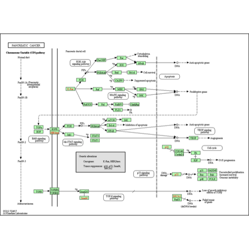
There is much to explore, and the KEGGREST package vignette provides examples. As a last illustration, we can acquire a static image of the (human) pancreatic cancer pathway in which BRCA2 is implicated.
library(png)
library(grid)
brpng = keggGet("hsa05212", "image")
grid.raster(brpng)
Additional ontologies
The rols package interfaces to the EMBL-EBI Ontology Lookup Service.
library(rols)
oo = Ontologies()
oo
## Object of class 'Ontologies' with 198 entries
##    GENEPIO, MP ... SEPIO, SIBO
oo[[1]]
## Ontology: Genomic Epidemiology Ontology (genepio)
##   The Genomic Epidemiology Ontology (GenEpiO) covers vocabulary
##   necessary to identify, document and research foodborne pathogens
##   and associated outbreaks.
##    Loaded: 2017-04-10 Updated: 2017-10-20 Version: 2017-04-09
##    4351 terms  137 properties  38 individuals
To control the amount of network traffic involved in query retrieval, there are stages of search.
glis = OlsSearch("glioblastoma")
glis
## Object of class 'OlsSearch':
##   query: glioblastoma
##   requested: 20 (out of 502)
##   response(s): 0
res = olsSearch(glis)
dim(res)
## NULL
resdf = as(res, "data.frame") # get content
resdf[1:4,1:4]
##                                                     id
## 1 ncit:class:http://purl.obolibrary.org/obo/NCIT_C3058
## 2     omit:http://purl.obolibrary.org/obo/OMIT_0007102
## 3    ordo:class:http://www.orpha.net/ORDO/Orphanet_360
## 4   hp:class:http://purl.obolibrary.org/obo/HP_0100843
##                                           iri   short_form        label
## 1   http://purl.obolibrary.org/obo/NCIT_C3058   NCIT_C3058 Glioblastoma
## 2 http://purl.obolibrary.org/obo/OMIT_0007102 OMIT_0007102 Glioblastoma
## 3      http://www.orpha.net/ORDO/Orphanet_360 Orphanet_360 Glioblastoma
## 4   http://purl.obolibrary.org/obo/HP_0100843   HP_0100843 Glioblastoma
resdf[1,5] # full description for one instance
## [[1]]
## [1] "The most malignant astrocytic tumor (WHO grade IV).  It is composed of poorly differentiated neoplastic astrocytes and it is characterized by the presence of cellular polymorphism, nuclear atypia, brisk mitotic activity, vascular thrombosis, microvascular proliferation and necrosis. It typically affects adults and is preferentially located in the cerebral hemispheres. It may develop from diffuse astrocytoma WHO grade II or anaplastic astrocytoma (secondary glioblastoma, IDH-mutant), but more frequently, it manifests after a short clinical history de novo, without evidence of a less malignant precursor lesion (primary glioblastoma, IDH- wildtype). (Adapted from WHO)"
The ontologyIndex supports import of ontologies in the Open Biological Ontologies (OBO) format, and includes very efficient facilities for querying and visualizing ontological systems.
General gene set management
The GSEABase package has excellent infrastructure for managing gene sets and collections thereof. We illustrate by importing a glioblastoma-related gene set from MSigDb.
library(GSEABase)
glioG = getGmt(system.file("gmt/glioSets.gmt", package="ph525x"))
## Warning in readLines(con, ...): incomplete final line found on '/
## Library/Frameworks/R.framework/Versions/3.4/Resources/library/ph525x/gmt/
## glioSets.gmt'
glioG
## GeneSetCollection
##   names: BALDWIN_PRKCI_TARGETS_UP, BEIER_GLIOMA_STEM_CELL_DN, ..., ZHENG_GLIOBLASTOMA_PLASTICITY_UP (47 total)
##   unique identifiers: ADA, AQP9, ..., ZFP28 (3671 total)
##   types in collection:
##     geneIdType: NullIdentifier (1 total)
##     collectionType: NullCollection (1 total)
head(geneIds(glioG[[1]]))
## [1] "ADA" "AQP9" "ATP2B4" "ATP6V1G1" "CBX6" "CCDC165"
A unified, self-describing approach for model organisms
The OrganismDb packages simplify access to annotation. Queries that succeed against TxDb, and org.[Nn].eg.db can be directed at the OrganismDb object.
library(Homo.sapiens)
class(Homo.sapiens)
## [1] "OrganismDb"
## attr(,"package")
## [1] "OrganismDbi"
Homo.sapiens
## OrganismDb Object:
## # Includes GODb Object:  GO.db
## # With data about:  Gene Ontology
## # Includes OrgDb Object:  org.Hs.eg.db
## # Gene data about:  Homo sapiens
## # Taxonomy Id:  9606
## # Includes TxDb Object:  TxDb.Hsapiens.UCSC.hg19.knownGene
## # Transcriptome data about:  Homo sapiens
## # Based on genome:  hg19
## # The OrgDb gene id ENTREZID is mapped to the TxDb gene id GENEID .
tx = transcripts(Homo.sapiens)
## 'select()' returned 1:1 mapping between keys and columns
keytypes(Homo.sapiens)
##  [1] "ACCNUM"       "ALIAS"        "CDSID"        "CDSNAME"
##  [5] "DEFINITION"   "ENSEMBL"      "ENSEMBLPROT"  "ENSEMBLTRANS"
##  [9] "ENTREZID"     "ENZYME"       "EVIDENCE"     "EVIDENCEALL"
## [13] "EXONID"       "EXONNAME"     "GENEID"       "GENENAME"
## [17] "GO"           "GOALL"        "GOID"         "IPI"
## [21] "MAP"          "OMIM"         "ONTOLOGY"     "ONTOLOGYALL"
## [25] "PATH"         "PFAM"         "PMID"         "PROSITE"
## [29] "REFSEQ"       "SYMBOL"       "TERM"         "TXID"
## [33] "TXNAME"       "UCSCKG"       "UNIGENE"      "UNIPROT"
columns(Homo.sapiens)
##  [1] "ACCNUM"       "ALIAS"        "CDSCHROM"     "CDSEND"
##  [5] "CDSID"        "CDSNAME"      "CDSSTART"     "CDSSTRAND"
##  [9] "DEFINITION"   "ENSEMBL"      "ENSEMBLPROT"  "ENSEMBLTRANS"
## [13] "ENTREZID"     "ENZYME"       "EVIDENCE"     "EVIDENCEALL"
## [17] "EXONCHROM"    "EXONEND"      "EXONID"       "EXONNAME"
## [21] "EXONRANK"     "EXONSTART"    "EXONSTRAND"   "GENEID"
## [25] "GENENAME"     "GO"           "GOALL"        "GOID"
## [29] "IPI"          "MAP"          "OMIM"         "ONTOLOGY"
## [33] "ONTOLOGYALL"  "PATH"         "PFAM"         "PMID"
## [37] "PROSITE"      "REFSEQ"       "SYMBOL"       "TERM"
## [41] "TXCHROM"      "TXEND"        "TXID"         "TXNAME"
## [45] "TXSTART"      "TXSTRAND"     "TXTYPE"       "UCSCKG"
## [49] "UNIGENE"      "UNIPROT"
Platform-oriented annotation
By sorting information on the GPL information page at NCBI GEO, we see that the most commonly use oligonucleotide array platform (with 4760 series in the archive) is the Affy Human Genome U133 plus 2.0 array (GPL 570). We can work with the annotation for this array with the hgu133plus2.db package.
library(hgu133plus2.db)
##
hgu133plus2.db
## ChipDb object:
## | DBSCHEMAVERSION: 2.1
## | Db type: ChipDb
## | Supporting package: AnnotationDbi
## | DBSCHEMA: HUMANCHIP_DB
## | ORGANISM: Homo sapiens
## | SPECIES: Human
## | MANUFACTURER: Affymetrix
## | CHIPNAME: Human Genome U133 Plus 2.0 Array
## | MANUFACTURERURL: http://www.affymetrix.com/support/technical/byproduct.affx?product=hg-u133-plus
## | EGSOURCEDATE: 2015-Sep27
## | EGSOURCENAME: Entrez Gene
## | EGSOURCEURL: ftp://ftp.ncbi.nlm.nih.gov/gene/DATA
## | CENTRALID: ENTREZID
## | TAXID: 9606
## | GOSOURCENAME: Gene Ontology
## | GOSOURCEURL: ftp://ftp.geneontology.org/pub/go/godatabase/archive/latest-lite/
## | GOSOURCEDATE: 20150919
## | GOEGSOURCEDATE: 2015-Sep27
## | GOEGSOURCENAME: Entrez Gene
## | GOEGSOURCEURL: ftp://ftp.ncbi.nlm.nih.gov/gene/DATA
## | KEGGSOURCENAME: KEGG GENOME
## | KEGGSOURCEURL: ftp://ftp.genome.jp/pub/kegg/genomes
## | KEGGSOURCEDATE: 2011-Mar15
## | GPSOURCENAME: UCSC Genome Bioinformatics (Homo sapiens)
## | GPSOURCEURL: ftp://hgdownload.cse.ucsc.edu/goldenPath/hg19
## | GPSOURCEDATE: 2010-Mar22
## | ENSOURCEDATE: 2015-Jul16
## | ENSOURCENAME: Ensembl
## | ENSOURCEURL: ftp://ftp.ensembl.org/pub/current_fasta
## | UPSOURCENAME: Uniprot
## | UPSOURCEURL: http://www.uniprot.org/
## | UPSOURCEDATE: Thu Oct  1 23:31:58 2015
##
## Please see: help('select') for usage information
The basic purpose of this resource (and of all the instances of the ChipDb class) is to map between probeset identifiers and higher-level genomic annotation.
The detailed information on probes, the constituents of probe sets, is given in packages with names ending in ‘probe’.
library(hgu133plus2probe)
head(hgu133plus2probe)
##                    sequence    x   y Probe.Set.Name
## 1 CACCCAGCTGGTCCTGTGGATGGGA  718 317      1007_s_at
## 2 GCCCCACTGGACAACACTGATTCCT 1105 483      1007_s_at
## 3 TGGACCCCACTGGCTGAGAATCTGG  584 901      1007_s_at
## 4 AAATGTTTCCTTGTGCCTGCTCCTG  192 205      1007_s_at
## 5 TCCTTGTGCCTGCTCCTGTACTTGT  844 979      1007_s_at
## 6 TGCCTGCTCCTGTACTTGTCCTCAG  537 971      1007_s_at
##   Probe.Interrogation.Position Target.Strandedness
## 1                         3330           Antisense
## 2                         3443           Antisense
## 3                         3512           Antisense
## 4                         3563           Antisense
## 5                         3570           Antisense
## 6                         3576           Antisense
dim(hgu133plus2probe)
## [1] 604258 6
Mapping out a probe set identifier to gene-level information can reveal some interesting ambiguities:
select(hgu133plus2.db, keytype="PROBEID",
  columns=c("SYMBOL", "GENENAME", "PATH", "MAP"), keys="1007_s_at")
## 'select()' returned 1:many mapping between keys and columns
##     PROBEID  SYMBOL                                    GENENAME PATH
## 1 1007_s_at    DDR1 discoidin domain receptor tyrosine kinase 1 <NA>
## 2 1007_s_at MIR4640                               microRNA 4640 <NA>
##       MAP
## 1 6p21.33
## 2 6p21.33
Apparently this probe set includes sequence that may be used to quantify abundance of both an mRNA and a micro RNA. As a sanity check we see that the distinct symbols map to the same cytoband.
Summary
We have covered a lot of material, from the nucleotide to the pathway level. The Annotation “view” at bioconductor.org can always be visited to survey existing resources.