## Now getting the GODb Object directly

## Now getting the OrgDb Object directly

## Now getting the TxDb Object directly

Overview

In this document we work with a small set of ranges and illustrate basic intra-range operations reduce, disjoin, gaps. We then add strand and seqname information and show how resize and flank are useful for identifying TSS and promoter regions.

A simple set of ranges

ir <- IRanges(c(3, 8, 14, 15, 19, 34, 40),
  width = c(12, 6, 6, 15, 6, 2, 7))

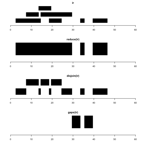
Let’s visualize ir and several intra-range operations.

par(mfrow=c(4,1), mar=c(4,2,2,2))
plotRanges(ir, xlim=c(0,60))
plotRanges(reduce(ir), xlim=c(0,60))
plotRanges(disjoin(ir), xlim=c(0,60))
plotRanges(gaps(ir), xlim=c(0,60))

reduce(x) produces a set of nonoverlapping ranges that cover all positions covered by x. This can be used to reduce complexity of a gene model with many transcripts, where we may just want the addresses of intervals known to be transcribed, regardless of transcript of residence.

disjoin(x) produces a set of ranges that cover all positions covered by x, such that none of the ranges in the disjoin output overlaps any end points of intervals in x. This gives us the largest possible collection of contiguous intervals that are separated wherever the original set of intervals had an endpoint.

gaps(x) produces a set of ranges covering the positions in [start(x), end(x)] that are not covered by any range in x. Given coding sequence addresses and exon intervals, this can be used to enumerate introns.

Extension to GRanges

We add chromosome and strand information.

library(GenomicRanges)
gir = GRanges(seqnames="chr1", ir, strand=c(rep("+", 4), rep("-",3)))

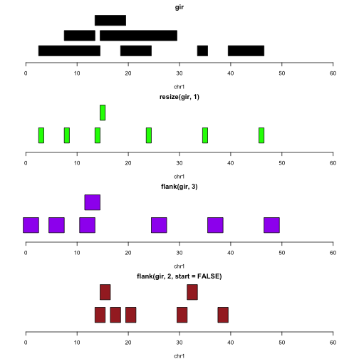
Let’s assume the intervals represent genes. The following plots illustrate the identification of transcription start sites (green), upstream promoter regions (purple), downstream promoter regions (brown).

par(mfrow=c(4,1), mar=c(4,2,2,2))
plotGRanges(gir, xlim=c(0,60))
plotGRanges(resize(gir,1), xlim=c(0,60),col="green")
plotGRanges(flank(gir,3), xlim=c(0,60), col="purple")
plotGRanges(flank(gir,2,start=FALSE), xlim=c(0,60), col="brown")

Note that we do not need to take special steps to deal with the differences in strand.