IRanges and GRanges
The IRanges and GRanges objects are core components of the Bioconductor infrastructure for defining integer ranges in general (IRanges), and specifically for addressing locations in the genome and hence including chromosome and strand information (GRanges). Here we will briefly explore what these objects are and a subset of the operations which manipulate IRanges and GRanges.
IRanges
First we load the IRanges package. This is included in the base installation of Bioconductor, but as with all Bioconductor packages it can be installed with biocLite. R will print out a bunch of messages when you load IRanges about objects which are masked from other packages. This is part of the normal loading process. Here we print these messages, although on some other book pages we suppress the messages for cleanliness:
library(IRanges)
The IRanges function defines interval ranges. If you provide it with two numbers, these are the start and end of a inclusive range, e.g. , which has width 6. When referring to the size of a range, the term width is used, instead of length.
ir <- IRanges(5,10)
ir
## IRanges object with 1 range and 0 metadata columns:
##           start       end     width
##       <integer> <integer> <integer>
##   [1]         5        10         6
start(ir)
## [1] 5
end(ir)
## [1] 10
width(ir)
## [1] 6
# for detailed information on the IRanges class:
# ?IRanges
A single IRanges object can hold more than one range. We do this by specifying vector to the start and end arguments.
IRanges(start=c(3,5,17), end=c(10,8,20))
## IRanges object with 3 ranges and 0 metadata columns:
##           start       end     width
##       <integer> <integer> <integer>
##   [1]         3        10         8
##   [2]         5         8         4
##   [3]        17        20         4
Intra-range operations
We will continue to work with the single range . We can look up a number of intra-range methods for IRanges objects, which mean that the operations work on each range independently. For example, we can shift all the ranges two integers to the left. By left and right, we refer to the direction on the integer number line: . Compare ir and shift(ir, -2):
# full details on the intra-range methods:
# ?"intra-range-methods"
ir
## IRanges object with 1 range and 0 metadata columns:
##           start       end     width
##       <integer> <integer> <integer>
##   [1]         5        10         6
shift(ir, -2)
## IRanges object with 1 range and 0 metadata columns:
##           start       end     width
##       <integer> <integer> <integer>
##   [1]         3         8         6
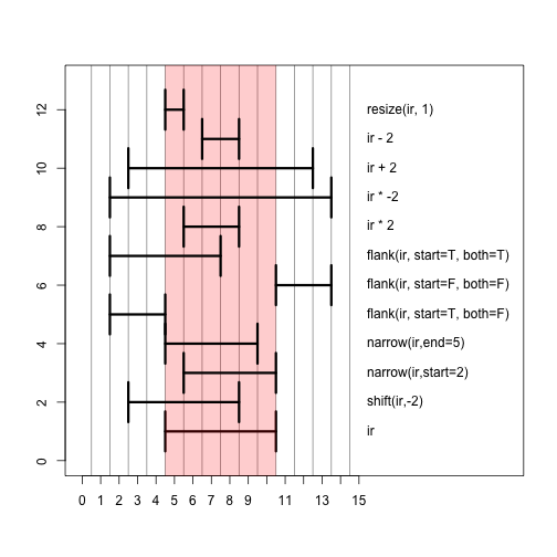
Here we show the result of a number of different operations applied to ir, with a picture below.
ir
## IRanges object with 1 range and 0 metadata columns:
##           start       end     width
##       <integer> <integer> <integer>
##   [1]         5        10         6
narrow(ir, start=2)
## IRanges object with 1 range and 0 metadata columns:
##           start       end     width
##       <integer> <integer> <integer>
##   [1]         6        10         5
narrow(ir, end=5)
## IRanges object with 1 range and 0 metadata columns:
##           start       end     width
##       <integer> <integer> <integer>
##   [1]         5         9         5
flank(ir, width=3, start=TRUE, both=FALSE)
## IRanges object with 1 range and 0 metadata columns:
##           start       end     width
##       <integer> <integer> <integer>
##   [1]         2         4         3
flank(ir, width=3, start=FALSE, both=FALSE)
## IRanges object with 1 range and 0 metadata columns:
##           start       end     width
##       <integer> <integer> <integer>
##   [1]        11        13         3
flank(ir, width=3, start=TRUE, both=TRUE)
## IRanges object with 1 range and 0 metadata columns:
##           start       end     width
##       <integer> <integer> <integer>
##   [1]         2         7         6
ir * 2
## IRanges object with 1 range and 0 metadata columns:
##           start       end     width
##       <integer> <integer> <integer>
##   [1]         6         8         3
ir * -2
## IRanges object with 1 range and 0 metadata columns:
##           start       end     width
##       <integer> <integer> <integer>
##   [1]         2        13        12
ir + 2
## IRanges object with 1 range and 0 metadata columns:
##           start       end     width
##       <integer> <integer> <integer>
##   [1]         3        12        10
ir - 2
## IRanges object with 1 range and 0 metadata columns:
##           start       end     width
##       <integer> <integer> <integer>
##   [1]         7         8         2
resize(ir, 1)
## IRanges object with 1 range and 0 metadata columns:
##           start       end     width
##       <integer> <integer> <integer>
##   [1]         5         5         1
Those same operations plotted in a single window. The red bar shows the shadow of the original range ir. The best way to get the hang of these operations is to try them out yourself in the console on ranges you define yourself.

Inter-range operations
There are also a set of inter-range methods. These are operations which work on a set of ranges, and the output depends on all the ranges, thus distinguishes these methods from the intra-range methods, for which the other ranges in the set do not change the output. This is best explained with some examples. The range function gives the integer range from the start of the leftmost range to the end of the rightmost range:
# full details on the inter-range methods:
# ?"inter-range-methods"
(ir <- IRanges(start=c(3,5,17), end=c(10,8,20)))
## IRanges object with 3 ranges and 0 metadata columns:
##           start       end     width
##       <integer> <integer> <integer>
##   [1]         3        10         8
##   [2]         5         8         4
##   [3]        17        20         4
range(ir)
## IRanges object with 1 range and 0 metadata columns:
##           start       end     width
##       <integer> <integer> <integer>
##   [1]         3        20        18
The reduce function collapses the ranges, so that integers are covered by only one range in the output.
reduce(ir)
## IRanges object with 2 ranges and 0 metadata columns:
##           start       end     width
##       <integer> <integer> <integer>
##   [1]         3        10         8
##   [2]        17        20         4
The gaps function gives back the ranges of integers which are in range(ir) but not covered by any of the ranges in ir:
gaps(ir)
## IRanges object with 1 range and 0 metadata columns:
##           start       end     width
##       <integer> <integer> <integer>
##   [1]        11        16         6
The disjoin function breaks up the ranges in ir into discrete ranges. This is best explained with examples, but here is the formal definition first:
returns a disjoint object, by finding the union of the end points in ‘x’. In other words, the result consists of a range for every interval, of maximal length, over which the set of overlapping ranges in ‘x’ is the same and at least of size 1.
disjoin(ir)
## IRanges object with 4 ranges and 0 metadata columns:
##           start       end     width
##       <integer> <integer> <integer>
##   [1]         3         4         2
##   [2]         5         8         4
##   [3]         9        10         2
##   [4]        17        20         4
Note that this is not a comprehensive list. Check the man pages we listed above, and the best way to get the hang of the functions is to try them out on some ranges you construct yourself. Note that most of the functions are defined both for IRanges and for GRanges, which will be described below.
GRanges
GRanges are objects which contain IRanges and two more important pieces of information:
- the chromosome we are referring to (called
seqnamesin Bioconductor) - the strand of DNA we are referring to
Strand can be specified as plus “+” or minus “-“, or left unspecified with “*”. Plus strand features have the biological direction from left to right on the number line, and minus strand features have the biological direction from right to left. In terms of the IRanges, plus strand features go from start to end, and minus strand features go from end to start. This may seem a bit confusing at first, but this is required because width is defined as end - start + 1, and negative width ranges are not allowed. Because DNA has two strands, which have an opposite directionality, strand is necessary for uniquely referring to DNA.
With an IRange, a chromosome name, and a strand, we can be sure we are uniquely referring to the same region and strand of the DNA molecule as another researcher, given that we are using the same build of genome. There are other pieces of information which can be contained within a GRanges object, but the two above are the most important.
library(GenomicRanges)
Let’s create a set of two ranges on a made-up chromosome, chrZ. And we will say that these ranges refer to the genome hg19. Because we have not linked our genome to a database, we are allowed to specify a chromosome which does not really exist in hg19.
gr <- GRanges("chrZ", IRanges(start=c(5,10),end=c(35,45)),
              strand="+", seqlengths=c(chrZ=100L))
gr
## GRanges object with 2 ranges and 0 metadata columns:
##       seqnames    ranges strand
##          <Rle> <IRanges>  <Rle>
##   [1]     chrZ  [ 5, 35]      +
##   [2]     chrZ  [10, 45]      +
##   -------
##   seqinfo: 1 sequence from an unspecified genome
genome(gr) <- "hg19"
gr
## GRanges object with 2 ranges and 0 metadata columns:
##       seqnames    ranges strand
##          <Rle> <IRanges>  <Rle>
##   [1]     chrZ  [ 5, 35]      +
##   [2]     chrZ  [10, 45]      +
##   -------
##   seqinfo: 1 sequence from hg19 genome
Note the seqnames and seqlengths which we defined in the call above:
seqnames(gr)
## factor-Rle of length 2 with 1 run
##   Lengths:    2
##   Values : chrZ
## Levels(1): chrZ
seqlengths(gr)
## chrZ
##  100
We can use the shift function as we did with the IRanges. However, notice the warning when we try to shift the range beyond the length of the chromosome:
shift(gr, 10)
## GRanges object with 2 ranges and 0 metadata columns:
##       seqnames    ranges strand
##          <Rle> <IRanges>  <Rle>
##   [1]     chrZ  [15, 45]      +
##   [2]     chrZ  [20, 55]      +
##   -------
##   seqinfo: 1 sequence from hg19 genome
shift(gr, 80)
## Warning in valid.GenomicRanges.seqinfo(x, suggest.trim = TRUE): GRanges object contains 2 out-of-bound ranges located on sequence
##   chrZ. Note that only ranges located on a non-circular sequence
##   whose length is not NA can be considered out-of-bound (use
##   seqlengths() and isCircular() to get the lengths and circularity
##   flags of the underlying sequences). You can use trim() to trim
##   these ranges. See ?`trim,GenomicRanges-method` for more
##   information.
## GRanges object with 2 ranges and 0 metadata columns:
##       seqnames    ranges strand
##          <Rle> <IRanges>  <Rle>
##   [1]     chrZ [85, 115]      +
##   [2]     chrZ [90, 125]      +
##   -------
##   seqinfo: 1 sequence from hg19 genome
If we trim the ranges, we obtain the ranges which are left, disregarding the portion that stretched beyond the length of the chromosome:
trim(shift(gr, 80))
## Warning in valid.GenomicRanges.seqinfo(x, suggest.trim = TRUE): GRanges object contains 2 out-of-bound ranges located on sequence
##   chrZ. Note that only ranges located on a non-circular sequence
##   whose length is not NA can be considered out-of-bound (use
##   seqlengths() and isCircular() to get the lengths and circularity
##   flags of the underlying sequences). You can use trim() to trim
##   these ranges. See ?`trim,GenomicRanges-method` for more
##   information.
## GRanges object with 2 ranges and 0 metadata columns:
##       seqnames    ranges strand
##          <Rle> <IRanges>  <Rle>
##   [1]     chrZ [85, 100]      +
##   [2]     chrZ [90, 100]      +
##   -------
##   seqinfo: 1 sequence from hg19 genome
We can add columns of information to each range using the mcols function (stands for metadata columns). Note: this is also possible with IRanges. We can remove the columns by assigning NULL.
mcols(gr)
## DataFrame with 2 rows and 0 columns
mcols(gr)$value <- c(-1,4)
gr
## GRanges object with 2 ranges and 1 metadata column:
##       seqnames    ranges strand |     value
##          <Rle> <IRanges>  <Rle> | <numeric>
##   [1]     chrZ  [ 5, 35]      + |        -1
##   [2]     chrZ  [10, 45]      + |         4
##   -------
##   seqinfo: 1 sequence from hg19 genome
mcols(gr)$value <- NULL
GRangesList
Especially when referring to genes, it is useful to create a list of GRanges. This is useful for representing groupings, for example the exons which belong to each gene. The elements of the list are the genes, and within each element the exon ranges are defined as GRanges.
gr2 <- GRanges("chrZ",IRanges(11:13,51:53))
grl <- GRangesList(gr, gr2)
grl
## GRangesList object of length 2:
## [[1]]
## GRanges object with 2 ranges and 0 metadata columns:
##       seqnames    ranges strand
##          <Rle> <IRanges>  <Rle>
##   [1]     chrZ  [ 5, 35]      +
##   [2]     chrZ  [10, 45]      +
##
## [[2]]
## GRanges object with 3 ranges and 0 metadata columns:
##       seqnames   ranges strand
##   [1]     chrZ [11, 51]      *
##   [2]     chrZ [12, 52]      *
##   [3]     chrZ [13, 53]      *
##
## -------
## seqinfo: 1 sequence from hg19 genome
The length of the GRangesList is the number of GRanges object within. To get the length of each GRanges we call elementNROWS. We can index into the list using typical list indexing of two square brackets.
length(grl)
## [1] 2
elementNROWS(grl)
## [1] 2 3
grl[[1]]
## GRanges object with 2 ranges and 0 metadata columns:
##       seqnames    ranges strand
##          <Rle> <IRanges>  <Rle>
##   [1]     chrZ  [ 5, 35]      +
##   [2]     chrZ  [10, 45]      +
##   -------
##   seqinfo: 1 sequence from hg19 genome
If we ask the width, the result is an IntegerList. If we apply sum, we get a numeric vector of the sum of the widths of each GRanges object in the list.
width(grl)
## IntegerList of length 2
## [[1]] 31 36
## [[2]] 41 41 41
sum(width(grl))
## [1] 67 123
We can add metadata columns as before, now one row of metadata for each GRanges object, not for each range. It doesn’t show up when we print the GRangesList, but it is still stored and accessible with mcols.
mcols(grl)$value <- c(5,7)
grl
## GRangesList object of length 2:
## [[1]]
## GRanges object with 2 ranges and 0 metadata columns:
##       seqnames    ranges strand
##          <Rle> <IRanges>  <Rle>
##   [1]     chrZ  [ 5, 35]      +
##   [2]     chrZ  [10, 45]      +
##
## [[2]]
## GRanges object with 3 ranges and 0 metadata columns:
##       seqnames   ranges strand
##   [1]     chrZ [11, 51]      *
##   [2]     chrZ [12, 52]      *
##   [3]     chrZ [13, 53]      *
##
## -------
## seqinfo: 1 sequence from hg19 genome
mcols(grl)
## DataFrame with 2 rows and 1 column
##       value
##   <numeric>
## 1         5
## 2         7
findOverlaps and %over%
We will demonstrate two commonly used methods for comparing GRanges objects. First we build two sets of ranges:
(gr1 <- GRanges("chrZ",IRanges(c(1,11,21,31,41),width=5),strand="*"))
## GRanges object with 5 ranges and 0 metadata columns:
##       seqnames    ranges strand
##          <Rle> <IRanges>  <Rle>
##   [1]     chrZ  [ 1,  5]      *
##   [2]     chrZ  [11, 15]      *
##   [3]     chrZ  [21, 25]      *
##   [4]     chrZ  [31, 35]      *
##   [5]     chrZ  [41, 45]      *
##   -------
##   seqinfo: 1 sequence from an unspecified genome; no seqlengths
(gr2 <- GRanges("chrZ",IRanges(c(19,33),c(38,35)),strand="*"))
## GRanges object with 2 ranges and 0 metadata columns:
##       seqnames    ranges strand
##          <Rle> <IRanges>  <Rle>
##   [1]     chrZ  [19, 38]      *
##   [2]     chrZ  [33, 35]      *
##   -------
##   seqinfo: 1 sequence from an unspecified genome; no seqlengths
findOverlaps returns a Hits object which contains the information about which ranges in the query (the first argument) overlapped which ranges in the subject (the second argument). There are many options for specifying what kind of overlaps should be counted.
fo <- findOverlaps(gr1, gr2)
fo
## Hits object with 3 hits and 0 metadata columns:
##       queryHits subjectHits
##       <integer>   <integer>
##   [1]         3           1
##   [2]         4           1
##   [3]         4           2
##   -------
##   queryLength: 5 / subjectLength: 2
queryHits(fo)
## [1] 3 4 4
subjectHits(fo)
## [1] 1 1 2
Another way of getting at overlap information is to use %over% which returns a logical vector of which ranges in the first argument overlapped any ranges in the second.
gr1 %over% gr2
## [1] FALSE FALSE TRUE TRUE FALSE
gr1[gr1 %over% gr2]
## GRanges object with 2 ranges and 0 metadata columns:
##       seqnames    ranges strand
##          <Rle> <IRanges>  <Rle>
##   [1]     chrZ  [21, 25]      *
##   [2]     chrZ  [31, 35]      *
##   -------
##   seqinfo: 1 sequence from an unspecified genome; no seqlengths
Note that both of these are strand-specific, although findOverlaps has an ignore.strand option.
gr1 <- GRanges("chrZ",IRanges(1,10),strand="+")
gr2 <- GRanges("chrZ",IRanges(1,10),strand="-")
gr1 %over% gr2
## [1] FALSE
Rle and Views
Lastly, we give you a short glimpse into two related classes defined in IRanges, the Rle and Views classes. Rle stands for run-length encoding, which is a form of compression for repetitive data. Instead of storing: , we would store the number 1, and the number of repeats: 4. The more repetitive the data, the greater the compression with Rle.
We use str to examine the internal structure of the Rle, to show it is only storing the numeric values and the number of repeats
(r <- Rle(c(1,1,1,0,0,-2,-2,-2,rep(-1,20))))
## numeric-Rle of length 28 with 4 runs
##   Lengths:  3  2  3 20
##   Values :  1  0 -2 -1
str(r)
## Formal class 'Rle' [package "S4Vectors"] with 4 slots
##   ..@ values         : num [1:4] 1 0 -2 -1
##   ..@ lengths        : int [1:4] 3 2 3 20
##   ..@ elementMetadata: NULL
##   ..@ metadata       : list()
as.numeric(r)
##  [1]  1  1  1  0  0 -2 -2 -2 -1 -1 -1 -1 -1 -1 -1 -1 -1 -1 -1 -1 -1 -1 -1
## [24] -1 -1 -1 -1 -1
A Views object can be thought of as “windows” looking into a sequence.
(v <- Views(r, start=c(4,2), end=c(7,6)))
## Views on a 28-length Rle subject
##
## views:
##     start end width
## [1]     4   7     4 [ 0  0 -2 -2]
## [2]     2   6     5 [ 1  1  0  0 -2]
Note that the internal structure of the Views object is just the original object, and the IRanges which specify the windows. The great benefit of Views is when the original object is not stored in memory, in which case the Views object is a lightweight class which helps us reference subsequences, without having to load the entire sequence into memory.
str(v)
## Formal class 'RleViews' [package "IRanges"] with 5 slots
##   ..@ subject        :Formal class 'Rle' [package "S4Vectors"] with 4 slots
##   .. .. ..@ values         : num [1:4] 1 0 -2 -1
##   .. .. ..@ lengths        : int [1:4] 3 2 3 20
##   .. .. ..@ elementMetadata: NULL
##   .. .. ..@ metadata       : list()
##   ..@ ranges         :Formal class 'IRanges' [package "IRanges"] with 6 slots
##   .. .. ..@ start          : int [1:2] 4 2
##   .. .. ..@ width          : int [1:2] 4 5
##   .. .. ..@ NAMES          : NULL
##   .. .. ..@ elementType    : chr "integer"
##   .. .. ..@ elementMetadata: NULL
##   .. .. ..@ metadata       : list()
##   ..@ elementType    : chr "ANY"
##   ..@ elementMetadata: NULL
##   ..@ metadata       : list()
Applications with genomic elements: strand-aware operations
In this document we work with a small set of ranges and illustrate basic intra-range operations reduce, disjoin, gaps. We then add strand and seqname information and show how resize and flank are useful for identifying TSS and promoter regions.
A simple set of ranges
ir <- IRanges(c(3, 8, 14, 15, 19, 34, 40),
  width = c(12, 6, 6, 15, 6, 2, 7))
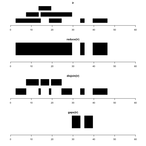
Let’s visualize ir and several intra-range operations.
par(mfrow=c(4,1), mar=c(4,2,2,2))
plotRanges(ir, xlim=c(0,60))
plotRanges(reduce(ir), xlim=c(0,60))
plotRanges(disjoin(ir), xlim=c(0,60))
plotRanges(gaps(ir), xlim=c(0,60))

reduce(x) produces a set of nonoverlapping ranges that cover all positions covered by x. This can be used to reduce complexity of a gene model with many transcripts, where we may just want the addresses of intervals known to be transcribed, regardless of transcript of residence.
disjoin(x) produces a set of ranges that cover all positions covered by x, such that none of the ranges in the disjoin output overlaps any end points of intervals in x. This gives us the largest possible collection of contiguous intervals that are separated wherever the original set of intervals had an endpoint.
gaps(x) produces a set of ranges covering the positions in [start(x), end(x)] that are not covered by any range in x. Given coding sequence addresses and exon intervals, this can be used to enumerate introns.
Extension to GRanges
We add chromosome and strand information.
library(GenomicRanges)
gir = GRanges(seqnames="chr1", ir, strand=c(rep("+", 4), rep("-",3)))
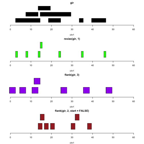
Let’s assume the intervals represent genes. The following plots illustrate the identification of transcription start sites (green), upstream promoter regions (purple), downstream promoter regions (brown).
par(mfrow=c(4,1), mar=c(4,2,2,2))
plotGRanges(gir, xlim=c(0,60))
plotGRanges(resize(gir,1), xlim=c(0,60),col="green")
plotGRanges(flank(gir,3), xlim=c(0,60), col="purple")
plotGRanges(flank(gir,2,start=FALSE), xlim=c(0,60), col="brown")

Note that we do not need to take special steps to deal with the differences in strand.
Applications to visualization of methylation array data
In our discussion of SummarizedExperiment applications, we imported data generated using an Illumina 450k methylation array.
In this section we’ll indicate how to use GenomicRanges and Gviz to explore methylation patterns in the context of gene-level annotation. The idea is simple: just extract the M-values (log-scaled locus-specific estimates of ratio of methylated to total DNA) from all samples and plot them in the context of gene models for selected genes.
We recall how the data were acquired and imported:
library(ArrayExpress)
if (!file.exists("E-MTAB-5797.sdrf.txt")) nano = getAE("E-MTAB-5797")
library(minfi)
pref = unique(substr(dir(patt="idat"),1,17)) # find the prefix strings
raw = read.metharray(pref)
glioMeth = preprocessQuantile(raw) # generate SummarizedExperiment
## [preprocessQuantile] Mapping to genome.
## [preprocessQuantile] Fixing outliers.
## [preprocessQuantile] Quantile normalizing.
Those steps require an internet connection and take just a few minutes.
Once we have glioMeth in our session, add the following
code to your session too. We will discuss how it works below.
MbyGene = function(mset, symbol="TP53", rad=5000) {
# phase 1: annotated GRanges for the gene
 require(erma)
 require(Gviz)
 gmod = suppressMessages(genemodel(symbol))     # erma utility
 gseq = as.character(seqnames(gmod)[1])
 gmod$transcript = symbol
# phase 2: filter down to the region of interest
 mlim = mset[which(seqnames(mset)==gseq),] # restrict to chromosome
 # now focus the methylation data to vicinity of gene
 d1 = subsetByOverlaps(GRanges(rowRanges(mlim),,, getM(mlim)),
         range(gmod)+rad)
# phase 3: use Gviz
 plotTracks(list(DataTrack(d1),
              GeneRegionTrack(gmod,
               transcriptAnnotation="transcript", name=gseq),
              GenomeAxisTrack(name=gseq, showTitle=TRUE)))
}
The comments to the code indicate the three phases: acquire
gene region and add the transcript annotation for
informative plotting of the union of all exons; reduce
the GenomicRatioSet (which inherits from RangedSummarizedExperiment)
to the interval of interest, determined by both the
gene model and the rad argument; use Gviz to construct
plottable objects and plot them.
The details of Gviz are well-documented in the user manual for that package. We will return to the topic in the 6x component of this series. However, if you have entered the code correctly, you can generate gene-centric plots as follows:
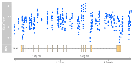
MbyGene(glioMeth, symbol="TERT")

The display allows us to see
- The genomic context (chromosome and region in megabase units)
- The structure of the gene of interest in a single line, representing a union of expressed intervals
- The locations of 450k probes (x coordinates of data points in blue)
- The between-sample variation in methylation estimates
- The variation of methylation across the genomic region selected
In the 6x module we will learn how to use additional packages to create an interactive display of this type, allowing us to select genes and zoom into regions of interest ad libitum.
Footnotes
For more information about the GenomicRanges package, check out the PLOS Comp Bio paper, which the authors of GenomicRanges published:
http://www.ploscompbiol.org/article/info%3Adoi%2F10.1371%2Fjournal.pcbi.1003118
Also the software vignettes have a lot of details about the functionality. Check out the “An Introduction to GenomicRanges” vignette. All of the vignette PDFs are available here:
browseVignettes("GenomicRanges")
Or the help pages here:
help(package="GenomicRanges", help_type="html")
For users of bedtools, the HelloRanges package is useful for converting concepts between BED and GRanges conceptual frameworks.