Introduction (revised October 2017)

It is very common for life scientists to use spreadsheets to record and manage experimental data. In these problems we will build up a discipline of data management for genome-scale experiments using R and Bioconductor.

It may seem unusual to recommend R-based software for managing data. Ordinarily R is used for programming and computing statistical analyses. However, Bioconductor has taken very seriously the need to carefully annotate, in a unified way, many aspects of complex biological experiments. This approach allows us to import assay outputs (such as multiple microarray scans, or multiple sequencing alignments), combining them with relevant metadata about the experiment and the samples assayed, saving all the information in a single R variable. By carefully designing the structure of this variable, programs can operate reliably on various aspects of the data. Ultimately a more efficient management and analysis environment is obtained.

We will come to understand this enhancement of efficiency by working from some very basic representations of experimental data, proceeding stepwise to more advanced integrative representations that are the hallmark of Bioconductor’s approach to genome-scale data.

Illustrative exercises (worked through in video)

1.0 Distinct components from an experiment.

library(GSE5859Subset)
library(Biobase)
.oldls = ls()
data(GSE5859Subset)
.newls = ls()

The objects obtained from the data() command are

newstuff = setdiff(.newls, .oldls)
newstuff

## [1] "geneAnnotation" "geneExpression" "sampleInfo"

and they have classes

cls = lapply(newstuff, function(x) class(get(x)))
names(cls) = newstuff
cls

## $$geneAnnotation
## [1] "data.frame"
## 
## $$geneExpression
## [1] "matrix"
## 
## $$sampleInfo
## [1] "data.frame"

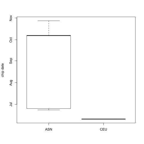
It is easy to make an informative plot of hybridization date by ethnicity of sample source using standard R:

boxplot(date~factor(ethnicity), data=sampleInfo, ylab="chip date")

plot of chunk lket

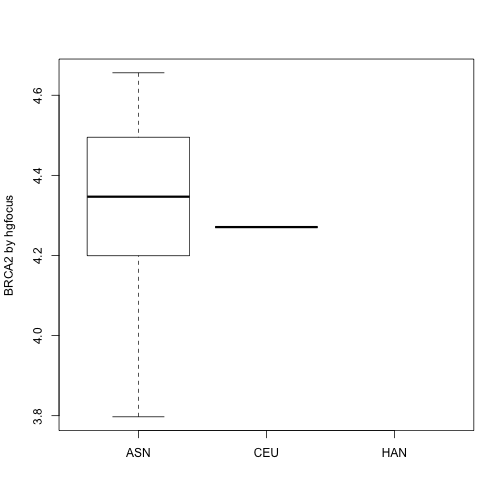
What if we want to look at expression of the gene BRCA2 by ethnicity? We have to do several things:

We need to determine which row of geneExpression corresponds to BRCA2, and to do this we need to know which column of geneAnnotation provides the information;
We need to ensure that the gene expression data in the matrix geneExpression are ordered consistently with the ordering of data in sampleInfo, and to do this we need to know which column of sampleInfo identifies the samples using the same tags as geneExpression.

Therefore, to relate gene expression to a sample characteristic we need to manipulate three different entities (expression, sample annotation, and gene annotation), ensuring that they are properly coordinated.

all.equal(colnames(geneExpression), sampleInfo$filename)

## [1] TRUE

all.equal(rownames(geneExpression), geneAnnotation$PROBEID)

## [1] TRUE

ind = which(geneAnnotation$SYMBOL=="BRCA2")
boxplot(geneExpression[ind,]~sampleInfo$ethnicity, ylab="BRCA2 by hgfocus")

plot of chunk dochks

It works, but it is complicated. To reduce complexity, Bioconductor defines ExpressionSet.

1.1 The ExpressionSet container.

There are high-level commands that simplify ExpressionSet construction.

es1 = ExpressionSet(geneExpression)
pData(es1) = sampleInfo
fData(es1) = geneAnnotation
es1

## ExpressionSet (storageMode: lockedEnvironment)
## assayData: 8793 features, 24 samples 
##   element names: exprs 
## protocolData: none
## phenoData
##   sampleNames: 107 122 ... 159 (24 total)
##   varLabels: ethnicity date filename group
##   varMetadata: labelDescription
## featureData
##   featureNames: 1 30 ... 12919 (8793 total)
##   fvarLabels: PROBEID CHR CHRLOC SYMBOL
##   fvarMetadata: labelDescription
## experimentData: use 'experimentData(object)'
## Annotation:

When we mention es1 we get a compact representation of lots of information about the experiment. Use es1 to visualize the confounding of hybridization date with ethnicity:

boxplot(es1$date~es1$ethnicity)

Now you’ve been introduced to the ExpressionSet container design and you’ve even constructed an ExpressionSet instance. We’ll use a more comprehensive representation of the data in the underlying experiment in the next task. We’ll use

library(GSE5859)
data(GSE5859)
e

## ExpressionSet (storageMode: lockedEnvironment)
## assayData: 8793 features, 208 samples 
##   element names: exprs, se.exprs 
## protocolData
##   sampleNames: GSM25349.CEL.gz GSM25350.CEL.gz ...
##     GSM136729.CEL.gz (208 total)
##   varLabels: ScanDate
##   varMetadata: labelDescription
## phenoData
##   sampleNames: 1 2 ... 208 (208 total)
##   varLabels: ethnicity date filename
##   varMetadata: labelDescription
## featureData: none
## experimentData: use 'experimentData(object)'
## Annotation: hgfocus

1.2 Metadata management. It is useful to have information about an experiment’s intentions and methods ready-to-hand. Some of the arrays used for GSE5859 were produced for a 2004 paper with Pubmed ID 15269782. We can, if connected to the internet, import information about that paper into R.

library(annotate)
p = pmid2MIAME("15269782")
p

## Experiment data
##   Experimenter name: Morley M 
##   Laboratory: NA 
##   Contact information:  
##   Title: Genetic analysis of genome-wide variation in human gene expression. 
##   URL:  
##   PMIDs: 15269782 
## 
##   Abstract: A 167 word abstract is available. Use 'abstract' method.

Check the display of e in your session. Then Use the command experimentData(e) <- p. How has the display of e changed? What is the result of experimentData(e)?

ExpressionSet: Why? and How?

We have moved fairly quickly through the creation and use of an ExpressionSet instance to illustrate some of its virtues. We will now provide some details on why and how this structure is designed and used.

Motivations underlying the ExpressionSet design are many. A few of the most important are

to reduce complexity of programming with complex assay, annotation, and sample-level information,
to support simple and idiomatic filtering of features and samples,
to control memory consumption as assay data are passed to analytical functions.

So much for “why”, to this point. “How” takes us for an excursion in software design strategy: object-oriented programming in R with the class system known as S4.

Object-oriented programming and S4 classes

Object-oriented programming (OOP) is a discipline of computer programming that helps to reduce program complexity and maintenance requirements, and to enhance program interoperability. There are various approaches to OOP, even within R, and we focus on the one known as S4. The basic idea is that an object

brings together data of different types in a unified structure,
is identified as a member of a formally specified class, and may be formally situated in a system of related objects,
“responds to” generic method calls in a class-specific way.

We can see the class structure for an ExpressionSet with getClass:

getClass("ExpressionSet")

## Class "ExpressionSet" [package "Biobase"]
## 
## Slots:
##                                                                
## Name:      experimentData          assayData          phenoData
## Class:              MIAME          AssayData AnnotatedDataFrame
##                                                                
## Name:         featureData         annotation       protocolData
## Class: AnnotatedDataFrame          character AnnotatedDataFrame
##                          
## Name:   .__classVersion__
## Class:           Versions
## 
## Extends: 
## Class "eSet", directly
## Class "VersionedBiobase", by class "eSet", distance 2
## Class "Versioned", by class "eSet", distance 3

This shows that there are 7 ‘slots’ comprising the class definition. Only the annotation slot is occupied by a simple R data type. All the other slots are to be occupied by instances of other S4 classes (or more basic R data types).

As an example, the MIAME class has the following definition:

getClass("MIAME")

## Class "MIAME" [package "Biobase"]
## 
## Slots:
##                                                             
## Name:               name               lab           contact
## Class:         character         character         character
##                                                             
## Name:              title          abstract               url
## Class:         character         character         character
##                                                             
## Name:          pubMedIds           samples    hybridizations
## Class:         character              list              list
##                                                             
## Name:       normControls     preprocessing             other
## Class:              list              list              list
##                         
## Name:  .__classVersion__
## Class:          Versions
## 
## Extends: 
## Class "MIAxE", directly
## Class "characterORMIAME", directly
## Class "Versioned", by class "MIAxE", distance 2

So we see that S4 allows us to define new data structures that encapsulate diverse types of information. We could do this with the very general “list” structure provided by R. But S4 allows us to guarantee properties of our new structures so that programs defined for these structures do not have to “check” on what they are operating on. The checks are built in to the class system.

DataFrame: an enhanced structure for tabular data

We are familiar with the data.frame structure from base R. Bioconductor introduced the DataFrame class to provide some additional capabilities that will be heavily exploited later.

library(S4Vectors)
sa2 = DataFrame(sampleInfo)
sa2

## DataFrame with 24 rows and 4 columns
##     ethnicity       date         filename     group
##      <factor>     <Date>      <character> <numeric>
## 1         ASN 2005-06-23 GSM136508.CEL.gz         1
## 2         ASN 2005-06-27 GSM136530.CEL.gz         1
## 3         ASN 2005-06-27 GSM136517.CEL.gz         1
## 4         ASN 2005-10-28 GSM136576.CEL.gz         1
## 5         ASN 2005-10-07 GSM136566.CEL.gz         1
## ...       ...        ...              ...       ...
## 20        ASN 2005-06-27 GSM136524.CEL.gz         0
## 21        ASN 2005-06-23 GSM136514.CEL.gz         0
## 22        ASN 2005-10-07 GSM136563.CEL.gz         0
## 23        ASN 2005-10-07 GSM136564.CEL.gz         0
## 24        ASN 2005-10-07 GSM136572.CEL.gz         0

The show method depicts top and bottom table row data, provides information on column datatype, and has the capacity to manage complex data types in columns more effectively than data.frame. Here is the class definition:

getClass("DataFrame")

## Class "DataFrame" [package "S4Vectors"]
## 
## Slots:
##                                                             
## Name:           rownames             nrows          listData
## Class: character_OR_NULL           integer              list
##                                                             
## Name:        elementType   elementMetadata          metadata
## Class:         character DataTable_OR_NULL              list
## 
## Extends: 
## Class "DataTable", directly
## Class "SimpleList", directly
## Class "DataTable_OR_NULL", by class "DataTable", distance 2
## Class "List", by class "SimpleList", distance 2
## Class "Vector", by class "SimpleList", distance 3
## Class "Annotated", by class "SimpleList", distance 4

Representations for mature archives from multisample NGS experiments

Short read sequencing leads to data collections that are more voluminous than gene-oriented microarray outputs.
Sequencing experiments may also be analyzed in more varied ways, so that it is valuable to provide efficient access to assay outputs at various levels of granularity.

A typical data flow for RNA-seq studies has phases 1) chromatographic display of base calls per cycle (seldom provided after, say, 2008), 2) base calls over the read length, with quality values, in FASTQ format, 3) feature quantification through statistical processing of genomic or transcriptomic alignments, 4) genome-scale archiving of multiple samples for inference on biologic questions of interest. FASTQ files are often developed in pairs for each sample.

A set of BAM files in Bioconductor

The RNAseqData.HNRNPC.bam.chr14 package includes BAM files derived from paired-end sequencing of 8 samples of HeLa cell lines, 4 of which were subjected to RNA interference to “knock down” the expression of the heterogeneous nuclear ribonucleoproteins C1 and C2 (denoted hnRNPC). This family of nuclear proteins is involved in pre-mRNA processing. We will demonstrate some approaches to managing the data from BAM to archived counts related to HNRNPC.

The BAM file pathnames are available in a character vector stored in the RNAseqData… package.

library(RNAseqData.HNRNPC.bam.chr14)
bfp = RNAseqData.HNRNPC.bam.chr14_BAMFILES
length(bfp)

## [1] 8

bfp[1]

##                                                                                                                ERR127306 
## "/Library/Frameworks/R.framework/Versions/3.4/Resources/library/RNAseqData.HNRNPC.bam.chr14/extdata/ERR127306_chr14.bam"

We use the Rsamtools package to manage these using a single variable.

library(Rsamtools)
bfl = BamFileList(file=bfp)
bfl

## BamFileList of length 8
## names(8): ERR127306 ERR127307 ERR127308 ... ERR127303 ERR127304 ERR127305

The BAM files include a limited amount of metadata about the genome to which the reads were aligned. This is propagated to the BamFileList instance.

seqinfo(bfl)

## Seqinfo object with 93 sequences from an unspecified genome:
##   seqnames              seqlengths isCircular genome
##   chr1                   249250621       <NA>   <NA>
##   chr10                  135534747       <NA>   <NA>
##   chr11                  135006516       <NA>   <NA>
##   chr11_gl000202_random      40103       <NA>   <NA>
##   chr12                  133851895       <NA>   <NA>
##   ...                          ...        ...    ...
##   chrUn_gl000247             36422       <NA>   <NA>
##   chrUn_gl000248             39786       <NA>   <NA>
##   chrUn_gl000249             38502       <NA>   <NA>
##   chrX                   155270560       <NA>   <NA>
##   chrY                    59373566       <NA>   <NA>

We see that the genome is “unspecified”, but we happen to know that the reference build ‘hg19’ was used to define the genomic sequence for alignment. [genome(bfl) <- “hg19” should rectify this but at present there is a bug. This should be fixed so that attempts to compare alignments using different references can be flagged or throw errors.]

In order to verify the success of the knockdown we will check the alignments in the vicinity of the genomic sequence coding for HNRNPC. Later we will show how to obtain the gene address using Bioconductor annotation tools; for now we just assert that for hg19

hnrnpcLoc = GRanges("chr14", IRanges(21677296, 21737638))
hnrnpcLoc

## GRanges object with 1 range and 0 metadata columns:
##       seqnames               ranges strand
##          <Rle>            <IRanges>  <Rle>
##   [1]    chr14 [21677296, 21737638]      *
##   -------
##   seqinfo: 1 sequence from an unspecified genome; no seqlengths

This identifies a region of chromosome 14 to which the HNRNPC coding gene is annotated for hg19. A simple way of assessing the expression quantifications uses summarizeOverlaps from the GenomicAlignments package. This counting method will implicitly use multicore computation.

library(GenomicAlignments)
library(BiocParallel)
register(SerialParam())
hnse = summarizeOverlaps(hnrnpcLoc,bfl)

Exercise

5.1 Examine the contents of the count component of hnse. What are the column identifiers for quantifications corresponding to the HNRNPC knockdown?

5.2 Add a variable condition with values knockdown and wildtype to the colData component of hnse.

5.3 Samples with identifier suffixes 306 and 307 are technical replicates of a single control sample; likewise for 308 and 309. Consequently there are six different biological samples in use. Add a variable to colData distinguishing these six samples.

Some intricacies of the ExpressionSet design (advanced)

Bioinformaticians work in an environment that is constantly changing. Computer capacity and throughput has increased dramatically since Bioconductor began (around 2000CE). The R language has also changed considerably. In the early days, it was important to be very economical about memory consumption, and R’s semantics at that time led to some inefficiencies through copying of objects in memory as they are passed to functions. Copying does not occur for R objects of class ‘environment’, and this led to the adoption of environments for storage of voluminous assay data.

class(slot(es1, "assayData"))

## [1] "environment"

ae = slot(es1, "assayData")
ae

## <environment: 0x7f813b4dc698>

This is a very special type of object for R. It can be thought of as a container for a reference to the matrix of expression values.

ls(ae)

## [1] "exprs"

dim(ae$exprs)

## [1] 8793   24

dim(exprs(es1))

## [1] 8793   24

object.size(ae)

## 56 bytes

object.size(ae$exprs)

## 2253824 bytes

Exercise (optional)

4.1. Explain the following findings.

e1 = new.env()
l1 = list()
e1$x = 5
l1$x = 5
all.equal(e1$x, l1$x)

## [1] TRUE

f = function(z) {z$x = 4; z$x}
all.equal(f(e1), f(l1))

## [1] TRUE

all.equal(e1$x, l1$x)  # different from before

## [1] "Mean relative difference: 0.25"

Management of genome-scale data