Understanding and building R packages

What is an R package?

Conceptually, an R package is a collection of functions, data objects, and documentation that coherently support a family of related data analysis operations.

Concretely, an R package is a structured collection of folders, organized and populated according to the rules of Writing R Extensions.

A new software package with `package.skeleton`

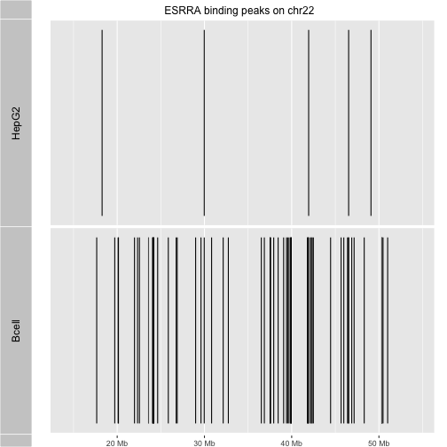
We can create our own packages using package.skeleton. We’ll illustrate that now with an enhancement to the ERBS package that was created for the course. We’ll create a new package that utilizes the peak data, defining a function juxta that allows us to compare binding peak patterns for the two cell types on a selected chromosome. (I have commented out code that uses an alternative graphics engine, for optional exploration.)

Here’s a definition of juxta. Add it to your R session.

juxta = function (chrname="chr22", ...) 
{
    require(ERBS)
    data(HepG2)
    data(GM12878)
    require(ggbio)
    require(GenomicRanges)  # "subset" is overused, need import detail
    ap1 = autoplot(HepG2[which(seqnames(HepG2)==chrname)])
    ap2 = autoplot(GM12878[which(seqnames(GM12878)==chrname)])
    tracks(HepG2 = ap1, Bcell = ap2, ...)
# alternative code for Gviz below
#    require(Gviz)
#    names(ap1) = "HepG2"
#    names(ap2) = "B-cell"
#    ax = GenomeAxisTrack()
#    plotTracks(list(ax, ap1, ap2))
}

Now demonstrate it as follows.

library(ERBS)
juxta("chr22", main="ESRRA binding peaks on chr22")

plot of chunk doj

In the video we will show how to use package.skeleton and the Rstudio editor to generate, document, and install this new package! We will not streamline the code in juxta to make use of inter-package symbol transfer by properly writing the DESCRIPTION and NAMESPACE files for the package, but leave this for an advanced course in software development.

A new annotation package with OrganismDbi

We have found the Homo.sapiens package to be quite convenient. We can get gene models, symbol to GO mappings, and so on, without remembering any more than keytypes, columns, keys, and select. At present there is no similar resource for S. cerevisiae. We can make one, following the OrganismDbi vignette. This is a very lightweight integrative package.

library(OrganismDbi)
gd = list( join1 = c(GO.db="GOID", org.Sc.sgd.db="GO"),
           join2 = c(org.Sc.sgd.db="ENTREZID",
              TxDb.Scerevisiae.UCSC.sacCer3.sgdGene="GENEID"))
if (!file.exists("Sac.cer3")) # don't do twice...
makeOrganismPackage(pkgname="Sac.cer3",  # simplify typing!
  graphData=gd, organism="Saccharomyces cerevisiae",
  version="1.0.0", maintainer="Student <ph525x@harvardx.edu>",
  author="Student <ph525x@harvardx.edu>",
  destDir=".",
  license="Artistic-2.0")

At this point we have a folder structure in our working folder that can support an installation.

install.packages("Sac.cer3", repos=NULL, type="source")
library(Sac.cer3)

## Loading required package: org.Sc.sgd.db

##

Sac.cer3

## OrganismDb Object:
## # Includes GODb Object:  GO.db 
## # With data about:  Gene Ontology 
## # Includes OrgDb Object:  org.Sc.sgd.db 
## # Gene data about:  Saccharomyces cerevisiae 
## # Taxonomy Id:  559292 
## # Includes TxDb Object:  TxDb.Scerevisiae.UCSC.sacCer3.sgdGene 
## # Transcriptome data about:  Saccharomyces cerevisiae 
## # Based on genome:  sacCer3 
## # The OrgDb gene id ENTREZID is mapped to the TxDb gene id GENEID .

columns(Sac.cer3)

##  [1] "ALIAS"        "CDSCHROM"     "CDSEND"       "CDSID"       
##  [5] "CDSNAME"      "CDSSTART"     "CDSSTRAND"    "COMMON"      
##  [9] "DEFINITION"   "DESCRIPTION"  "ENSEMBL"      "ENSEMBLPROT" 
## [13] "ENSEMBLTRANS" "ENTREZID"     "ENZYME"       "EVIDENCE"    
## [17] "EVIDENCEALL"  "EXONCHROM"    "EXONEND"      "EXONID"      
## [21] "EXONNAME"     "EXONRANK"     "EXONSTART"    "EXONSTRAND"  
## [25] "GENEID"       "GENENAME"     "GO"           "GOALL"       
## [29] "GOID"         "INTERPRO"     "ONTOLOGY"     "ONTOLOGYALL" 
## [33] "ORF"          "PATH"         "PFAM"         "PMID"        
## [37] "REFSEQ"       "SGD"          "SMART"        "TERM"        
## [41] "TXCHROM"      "TXEND"        "TXID"         "TXNAME"      
## [45] "TXSTART"      "TXSTRAND"     "TXTYPE"       "UNIPROT"

genes(Sac.cer3)

## GRanges object with 6534 ranges and 1 metadata column:
##             seqnames           ranges strand |       GENEID
##                <Rle>        <IRanges>  <Rle> | <FactorList>
##       Q0010     chrM   [ 3952,  4415]      + |        Q0010
##       Q0032     chrM   [11667, 11957]      + |        Q0032
##       Q0055     chrM   [13818, 26701]      + |        Q0055
##       Q0075     chrM   [24156, 25255]      + |        Q0075
##       Q0080     chrM   [27666, 27812]      + |        Q0080
##         ...      ...              ...    ... .          ...
##     YPR200C   chrXVI [939279, 939671]      - |      YPR200C
##     YPR201W   chrXVI [939922, 941136]      + |      YPR201W
##     YPR202W   chrXVI [943032, 944188]      + |      YPR202W
##   YPR204C-A   chrXVI [946856, 947338]      - |    YPR204C-A
##     YPR204W   chrXVI [944603, 947701]      + |      YPR204W
##   -------
##   seqinfo: 17 sequences (1 circular) from sacCer3 genome

Using devtools

Let’s use devtools to create a package centered around the juxta function. We will learn about roxygen too.

In the following code chunk, we use devtools::create to generate a package folder structure in a temporary directory.

curd = getwd()
kk = dir.create(tmpd <- tempfile()) # always new
setwd(tmpd)
library(devtools)
create("juxtaPack", list(Depends=c("ERBS", "ggbio"), 
    Description="Juxtapose ESRRA binding and gene models",
    Title="demonstration package"))

## Package: juxtaPack
## Title: demonstration package
## Version: 0.0.0.9000
## Authors@R: person("First", "Last", email = "first.last@example.com", role = c("aut", "cre"))
## Description: Juxtapose ESRRA binding and gene models
## Depends: ERBS, ggbio
## License: What license is it under?
## Encoding: UTF-8
## LazyData: true

setwd("juxtaPack")

We are now in the top folder of the package hierarchy. We will create a text file with documentation (prefixed by hashtag single quote) in the roxygen2 format. The text vector jlines defines the content. (Usually you will create your documentation and function code in a text editor.)

setwd(tmpd)
setwd("juxtaPack")
jlines = 
"#' render a chromosome and locations of ESRRA binding sites
#' @param chrname character(1) giving UCSC chromosome name
#' @examples
#' juxta()
#' @export
juxta = function (chrname='chr22', ...) 
{
    require(ERBS)
    data(HepG2)
    data(GM12878)
    require(ggbio)
    require(GenomicRanges)
    ac = as.character
    ap1 = autoplot(HepG2[which(ac(seqnames(HepG2))==chrname)])
    ap2 = autoplot(GM12878[which(ac(seqnames(GM12878))==chrname)])
    tracks(HepG2 = ap1, Bcell = ap2, ...)
}
"

We descend to the R folder and write our text file.

setwd(tmpd)
setwd("juxtaPack")
setwd("R")
writeLines(jlines, "jux.R")

We ascend to the package root and run document and install to get access to the new package.

setwd(tmpd)
setwd("juxtaPack")
document()

## Updating juxtaPack documentation

## Loading juxtaPack

## Updating roxygen version in /private/var/folders/5_/14ld0y7s0vbg_z0g2c9l8v300000gr/T/Rtmprv6lu6/file99ae46a8f0f5/juxtaPack/DESCRIPTION

## Writing NAMESPACE
## Writing juxta.Rd

install()

## Installing juxtaPack

## '/Library/Frameworks/R.framework/Resources/bin/R' --no-site-file  \
##   --no-environ --no-save --no-restore --quiet CMD INSTALL  \
##   '/private/var/folders/5_/14ld0y7s0vbg_z0g2c9l8v300000gr/T/Rtmprv6lu6/file99ae46a8f0f5/juxtaPack'  \
##   --library='/Library/Frameworks/R.framework/Versions/3.4/Resources/library'  \
##   --install-tests

##

## Reloading installed juxtaPack

## 
## Attaching package: 'juxtaPack'

## The following object is masked _by_ '.GlobalEnv':
## 
##     juxta

setwd(curd) # go back to where you started
library(juxtaPack)
juxta

## function (chrname="chr22", ...) 
## {
##     require(ERBS)
##     data(HepG2)
##     data(GM12878)
##     require(ggbio)
##     require(GenomicRanges)  # "subset" is overused, need import detail
##     ap1 = autoplot(HepG2[which(seqnames(HepG2)==chrname)])
##     ap2 = autoplot(GM12878[which(seqnames(GM12878)==chrname)])
##     tracks(HepG2 = ap1, Bcell = ap2, ...)
## # alternative code for Gviz below
## #    require(Gviz)
## #    names(ap1) = "HepG2"
## #    names(ap2) = "B-cell"
## #    ax = GenomeAxisTrack()
## #    plotTracks(list(ax, ap1, ap2))
## }

In summary:

We have used writeLines to generate a combination of roxygen documentation and R code in the file jux.R, in folder R, which was created as a subfolder of folder juxtaPack.
We then changed to the juxtaPack folder and ran document() that will translate the roxygen lines to statements in NAMESPACE and to a .Rd file in man.
We then ran install() to install the package in R, returned to our initial folder, and used library(juxtaPack) to attach our new package.

Full development would include production of a vignette and a suite of unit tests, giving a meaningful basis for using check() in devtools.
In a more extensive course, these would be addressed, but you can learn about them yourself by looking at any Bioconductor package. A good example is IRanges, which has extensive unit testing. There are many other good examples.

Wrapping up

You are now in a good position to revisit the motivations and core values section of the course pages.

In that section we described the concepts of functional object-oriented programming and continuous integration as they pertain to the development of highly reliable and relevant software tools, used in a variety of subdomains of genome science. The software engineering and reproducible research underpinnings of the Bioconductor project are at the heart of its scientific impact. For a nice set of remarks on usability in upcoming cloud contexts, see this recent Nature Toolbox commentary.