Bioconductor for genome-scale data -- quick intro
The R language and its packages and repositories
This course assumes a good working knowledge of the R language. The Rstudio environment is recommended. If you are jumping directly to 5x, skipping 1x-4x, and want to work through a tutorial before proceeding, Try R is very comprehensive.
Why R?
Bioconductor is based on R. Three key reasons for this are:
- R is used by many statisticians and biostatisticians to create algorithms that advance our ability to understand complex experimental data.
- R is highly interoperable, and fosters reuse of software components written in other languages.
- R is portable to the key operating systems running on commodity computing equipment (Linux, MacOSX, Windows) and can be used immediately by beginners with access to any of these platforms.
In summary, R’s ease-of-use and central role in statistics and “data science” make it a natural choice for a tool-set for use by biologists and statisticians confronting genome-scale experimental data. Since the Bioconductor project’s inception in 2001, it has kept pace with growing volumes and complexity of data emerging in genome-scale biology.
Functional object-oriented programming
R combines functional and object-oriented programming paradigms.^[Chambers 2014]
- In functional programming, notation and program activity mimic the
concept of function in mathematics. For example
square = function(x) x^2is valid R code that defines the symbol
squareas a function that computes the second power of its input. The body of the function is the program codex^2, in whichxis a “free variable”. Oncesquarehas been defined in this way,square(3)has value9. We say thesquarefunction has been evaluated on argument3. In R, all computations proceed by evaluation of functions. - In object-oriented programming, a strong focus is placed upon formalizing data structure, and defining methods that take advantage of guarantees established through the formalism. This approach is quite natural but did not get well-established in practical computer programming until the 1990s. As an advanced example with Bioconductor, we will consider an approach to defining an “object” representing on the genome of Homo sapiens:
library(Homo.sapiens)
class(Homo.sapiens)
## [1] "OrganismDb"
## attr(,"package")
## [1] "OrganismDbi"
methods(class=class(Homo.sapiens))
##  [1] asBED                 asGFF                 cds
##  [4] cdsBy                 coerce<-              columns
##  [7] dbconn                dbfile                disjointExons
## [10] distance              exons                 exonsBy
## [13] extractUpstreamSeqs   fiveUTRsByTranscript  genes
## [16] getTxDbIfAvailable    intronsByTranscript   isActiveSeq
## [19] isActiveSeq<-         keys                  keytypes
## [22] mapIds                mapToTranscripts      metadata
## [25] microRNAs             promoters             resources
## [28] select                selectByRanges        selectRangesById
## [31] seqinfo               show                  taxonomyId
## [34] threeUTRsByTranscript transcripts           transcriptsBy
## [37] tRNAs                 TxDb                  TxDb<-
## see '?methods' for accessing help and source code
We say that Homo.sapiens is an instance of the OrganismDb
class. Every instance of this class will respond meaningfully
to the methods
listed above. Each method is implemented as an R function.
What the function does depends upon the class of its arguments.
Of special note at this juncture are the methods
genes, exons, transcripts which will yield information about
fundamental components of genomes.
These methods will succeed for human and
for other model organisms such as Mus musculus, S. cerevisiae,
C. elegans, and others for which the Bioconductor project and its contributors have defined OrganismDb representations.
R packages, modularity, continuous integration
This section can be skipped on a first reading.
Package structure
We can perform object-oriented functional programming with R by writing R code. A basic approach is to create “scripts” that define all the steps underlying processes of data import and analysis. When scripts are written in such a way that they only define functions and data structures, it becomes possible to package them for convenient distribution to other users confronting similar data management and data analysis problems.
The R software packaging protocol specifies how source code in R and other languages can be organized together with metadata and documentation to foster convenient testing and redistribution. For example, an early version of the package defining this document had the folder layout given below:
├── DESCRIPTION  (text file with metadata on provenance, licensing)
├── NAMESPACE    (text file defining imports and exports)
├── R            (folder for R source code)
├── README.md    (optional for github face page)
├── data         (folder for exemplary data)
├── man          (folder for detailed documentation)
├── tests        (folder for formal software testing code)
└── vignettes    (folder for high-level documentation)
    ├── biocOv1.Rmd
    ├── biocOv1.html
The packaging protocol document “Writing R Extensions” provides
full details. The R command R CMD build [foldername] will operate on the
contents of a package folder to create an archive that can
be added to an R installation using R CMD INSTALL [archivename].
The R studio system performs these tasks with GUI elements.
Modularity and formal interdependence of packages
The packaging protocol helps us to isolate software that performs a limited set of operations, and to identify the version of a program collection that is inherently changing over time. There is no objective way to determine whether a set of operations is the right size for packaging. Some very useful packages carry out only a small number of tasks, while others have very broad scope. What is important is that the package concept permits modularization of software. This is important in two dimensions: scope and time. Modularization of scope is important to allow parallel independent development of software tools that address distinct problems. Modularization in time is important to allow identification of versions of software whose behavior is stable.
Continuous integration: testing package correctness and interoperability
The figure below is a snapshot of the build report for the development branch of Bioconductor.
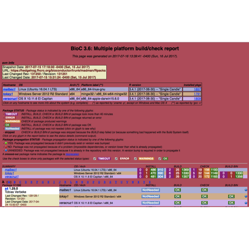
The six-column subtable in the upper half of the display includes a column “Installed pkgs”, with entry 1857 for the linux platform. This number varies between platforms and is generally increasing over time for the devel branch.
Putting it together
Bioconductor’s core developer group works hard to develop data structures that allow users to work conveniently with genomes and genome-scale data. Structures are devised to support the main phases of experimentation in genome scale biology:
- Parse large-scale assay data as produced by microarray or sequencer flow-cell scanners.
- Preprocess the (relatively) raw data to support reliable statistical interpretation.
- Combine assay quantifications with sample-level data to test hypotheses about relationships between molecular processes and organism-level characteristics such as growth, disease state.
In this course we will review the objects and functions that you can use to perform these and related tasks in your own research.
Basic premise and overview of 5x
You know to manipulate and analyze data using R, and you understand a considerable amount about statistical modeling. The Bioconductor project demonstrates that R is an effective vehicle for performing many – but not all – tasks that arise in genome-scale computational biology.
Some of the fundamental concepts that distinguish Bioconductor from other software systems addressing genome-scale data are
- use of object-oriented design concepts to unify disparate data types arising in genomic experiments;
- commitment to interoperable structures for genomic annotation, from nucleotide to population scale;
- continuous integration discipline for release and development cycles, withdaily testing on multiple widely used compute platforms. The purpose of this four-week module is to build appreciation for and expertise in the use of this system for many aspects of genome scale data analysis.
This module, 525.5x, breaks into four main pieces, with one week devoted to each of
- Motivation and techniques: what we measure and why, and how we manage the measurements with R
- Genomic annotation, with particular attention to the role of ranges in genomic coordinates in identifying genomic structures
- Preprocessing concepts for genome scale data, focusing on implementations in Bioconductor
- Testing genome-scale hypotheses with Bioconductor
Subsections of this chapter will sketch the concepts to be covered, along with some illustrative computations.
Motivation and techniques
The videos in “What we measure and why” provide schematic illustrations of the basic biological processes that can now be studied computationally. We noted that recipes for all the proteins that are fundamental to life processes of an organism are coded in the organism’s genomic DNA. Studies of differences between organisms, and certain changes within organisms (for example, development of tumors), often rely on computations involving genomic DNA sequence.
Bioconductor provides tools for working
directly with genomic DNA sequence for many organisms.
One basic approach uses computations on a “reference sequence”,
another focuses on differences between the genomic sequence
of a given individual, and the reference.
Reference sequence access
It is very easy to use Bioconductor to work with the reference sequence for Homo sapiens. Here we’ll have a look at chromosome 17.
library(BSgenome.Hsapiens.UCSC.hg19)
Hsapiens$chr17
##   81195210-letter "DNAString" instance
## seq: AAGCTTCTCACCCTGTTCCTGCATAGATAATTGC...GGTGTGGGTGTGGTGTGTGGGTGTGGGTGTGGT
Of note:
- the sequence is provided through an R package
- the name of the package indicates the curating source (UCSC) and reference version (hg19)
- familiar R syntax
$for selecting a list element is reused to select a chromosome
Representing DNA variants
A standard representation for individual departures from reference sequence
is Variant Call Format.
The VariantAnnotation package includes an example. We have two
high-level representations of some DNA variants – a summary of the
VCF content in the example, and the genomic addresses of
the sequence variants themselves.
fl <- system.file("extdata", "ex2.vcf", package="VariantAnnotation")
vcf <- readVcf(fl, "hg19")
vcf
## class: CollapsedVCF
## dim: 5 3
## rowRanges(vcf):
##   GRanges with 5 metadata columns: paramRangeID, REF, ALT, QUAL, FILTER
## info(vcf):
##   DataFrame with 6 columns: NS, DP, AF, AA, DB, H2
## info(header(vcf)):
##       Number Type    Description
##    NS 1      Integer Number of Samples With Data
##    DP 1      Integer Total Depth
##    AF A      Float   Allele Frequency
##    AA 1      String  Ancestral Allele
##    DB 0      Flag    dbSNP membership, build 129
##    H2 0      Flag    HapMap2 membership
## geno(vcf):
##   SimpleList of length 4: GT, GQ, DP, HQ
## geno(header(vcf)):
##       Number Type    Description
##    GT 1      String  Genotype
##    GQ 1      Integer Genotype Quality
##    DP 1      Integer Read Depth
##    HQ 2      Integer Haplotype Quality
rowRanges(vcf)
## GRanges object with 5 ranges and 5 metadata columns:
##                  seqnames             ranges strand | paramRangeID
##                     <Rle>          <IRanges>  <Rle> |     <factor>
##        rs6054257       20 [  14370,   14370]      * |         <NA>
##     20:17330_T/A       20 [  17330,   17330]      * |         <NA>
##        rs6040355       20 [1110696, 1110696]      * |         <NA>
##   20:1230237_T/.       20 [1230237, 1230237]      * |         <NA>
##        microsat1       20 [1234567, 1234569]      * |         <NA>
##                             REF                ALT      QUAL      FILTER
##                  <DNAStringSet> <DNAStringSetList> <numeric> <character>
##        rs6054257              G                  A        29        PASS
##     20:17330_T/A              T                  A         3         q10
##        rs6040355              A                G,T        67        PASS
##   20:1230237_T/.              T                           47        PASS
##        microsat1            GTC             G,GTCT        50        PASS
##   -------
##   seqinfo: 1 sequence from hg19 genome
Of note:
- the example data are “built-in” to the package, for illustration and testing
- the variable
vcfhas a concise display to the user - the variant locations, extracted using
rowRanges, are shown with a tag indicating their context in the hg19 reference build
Measures of gene expression
We’ll conclude this brief discussion of motivation and technique with a look at measurements on gene expression in the model organism Sacchomyces cerevisiae, baker’s yeast. A highly influential experiment undertook to use genome-wide measurement of mRNA abundance over a series of time points in the reproductive cycle. Again we use an R package to manage the data, and we use a special Bioconductor-defined data structure to provide access to information about the experiment and the results.
library(yeastCC)
data(spYCCES)
spYCCES
## ExpressionSet (storageMode: lockedEnvironment)
## assayData: 6178 features, 77 samples
##   element names: exprs
## protocolData: none
## phenoData
##   sampleNames: cln3_40 cln3_30 ... elu_390 (77 total)
##   varLabels: syncmeth time
##   varMetadata: labelDescription
## featureData: none
## experimentData: use 'experimentData(object)'
##   pubMedIds: 9843569
## Annotation:
experimentData(spYCCES)
## Experiment data
##   Experimenter name: Spellman PT
##   Laboratory: Department of Genetics, Stanford University Medical Center, Stanford, California 94306-5120, USA.
##   Contact information:
##   Title: Comprehensive identification of cell cycle-regulated genes of the yeast Saccharomyces cerevisiae by microarray hybridization.
##   URL:
##   PMIDs: 9843569
##
##   Abstract: A 150 word abstract is available. Use 'abstract' method.
After a bit of massaging, a topic on which you will become expert in the next few weeks, we can visualize the time course of a cell-cycle regulated gene.
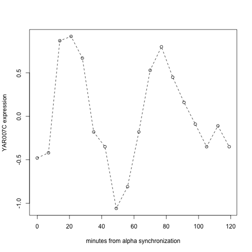
Of note:
- Informative metadata about the experiment are bound right to the data (pubmed ID and abstract accessible through
experimentData) - Simple syntax can be used to select components of complex experimental designs; in this case
spYCCES[, spYCCES$syncmeth=="alpha"]picks out just the colonies whose cell cycling was controlled using alpha pheromone - R’s plotting tools support general plot annotation and enhancement
- Statistical modeling tools to help distinguish cycling and non-cycling genes can be used immediately
Wrap-up
You’re about to engage with a few high-level lectures on genome structures and molecular biological techniques for measuring them. As you encounter these concepts, keep in mind what sorts of computations you consider relevant to understanding the structures and processes being studied. Find the tools to perform these computations in Bioconductor, and become expert in their use. And if you don’t find them, let us know, and perhaps we can point them out, or, if they don’t exist, build them together.