Distance and clustering lab

Let’s load the tissue gene expression data which Rafa discussed in the lecture:

# library(devtools) install_github('dagdata','genomicsclass')
library(dagdata)
data(tissuesGeneExpression)
library(Biobase)

## Loading required package: BiocGenerics
## Loading required package: methods
## Loading required package: parallel
## 
## Attaching package: 'BiocGenerics'
## 
## The following objects are masked from 'package:parallel':
## 
##     clusterApply, clusterApplyLB, clusterCall, clusterEvalQ,
##     clusterExport, clusterMap, parApply, parCapply, parLapply,
##     parLapplyLB, parRapply, parSapply, parSapplyLB
## 
## The following object is masked from 'package:stats':
## 
##     xtabs
## 
## The following objects are masked from 'package:base':
## 
##     anyDuplicated, append, as.data.frame, as.vector, cbind,
##     colnames, do.call, duplicated, eval, evalq, Filter, Find, get,
##     intersect, is.unsorted, lapply, Map, mapply, match, mget,
##     order, paste, pmax, pmax.int, pmin, pmin.int, Position, rank,
##     rbind, Reduce, rep.int, rownames, sapply, setdiff, sort,
##     table, tapply, union, unique, unlist
## 
## Welcome to Bioconductor
## 
##     Vignettes contain introductory material; view with
##     'browseVignettes()'. To cite Bioconductor, see
##     'citation("Biobase")', and for packages 'citation("pkgname")'.

rownames(tab) <- tab$filename
t <- ExpressionSet(e, AnnotatedDataFrame(tab))
t$Tissue <- factor(t$Tissue)
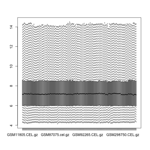
boxplot(exprs(t), range = 0)

plot of chunk unnamed-chunk-1

We will take the transpose of the vector, as the dist function will compute distances between the rows, and we want sample-sample distances: Note that the value in the 1,2 slot of the matrix of the object d is the same as the square root of the sum of squared differences, i.e., the definition of the Euclidean distance.

x <- t(exprs(t))
d <- dist(x)
class(d)

## [1] "dist"

as.matrix(d)[1, 2]

## [1] 85.85

sqrt(sum((x[1, ] - x[2, ])^2))

## [1] 85.85

Clustering

We can perform hierarchical clustering based on the distances defined above, using the hclust function. The plot method will make a plot of the tree that results from hclust.

hc <- hclust(d)
hc

## 
## Call:
## hclust(d = d)
## 
## Cluster method   : complete 
## Distance         : euclidean 
## Number of objects: 189

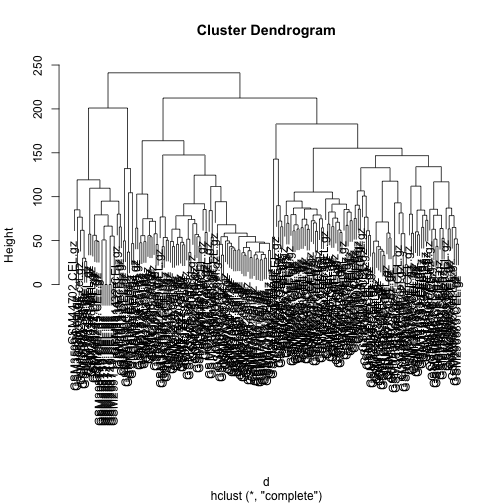
plot(hc)

plot of chunk unnamed-chunk-3

library(rafalib)

## Loading required package: RColorBrewer

mypar()
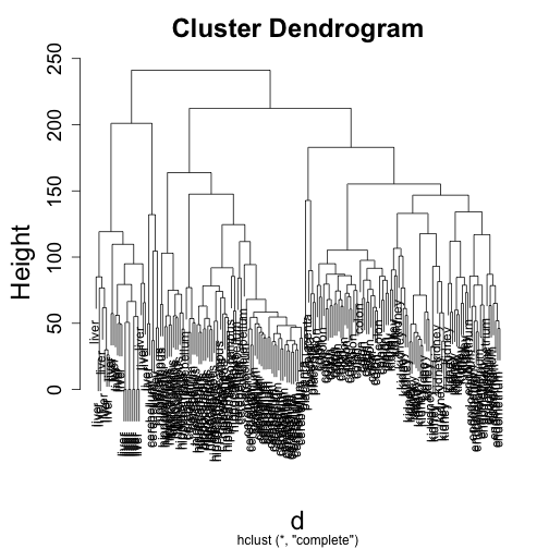
plot(hc, labels = t$Tissue)

plot of chunk unnamed-chunk-3

myplclust(hc, labels = t$Tissue, lab.col = as.fumeric(t$Tissue))
abline(h = 120)

plot of chunk unnamed-chunk-3

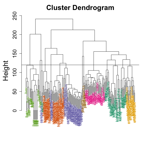
If we use the line above to cut the tree into clusters, we can examine how the clusters overlap with the actual tissues:

hclusters <- cutree(hc, h = 120)
table(true = t$Tissue, cluster = hclusters)

##              cluster
## true           1  2  3  4  5  6  7  8  9 10 11 12 13 14
##   cerebellum   0  0  0  0 31  0  0  0  2  0  0  5  0  0
##   colon        0  0  0  0  0  0 34  0  0  0  0  0  0  0
##   endometrium  0  0  0  0  0  0  0  0  0  0 15  0  0  0
##   hippocampus  0  0 12 19  0  0  0  0  0  0  0  0  0  0
##   kidney       9 18  0  0  0 10  0  0  2  0  0  0  0  0
##   liver        0  0  0  0  0  0  0 24  0  2  0  0  0  0
##   placenta     0  0  0  0  0  0  0  0  0  0  0  0  2  4

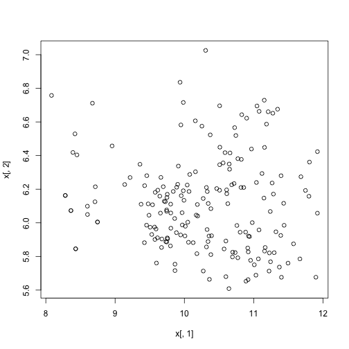
We can also call the kmeans function to perform k-means clustering as was explained in the lecture. Let’s run k-means on the samples in the space of the first two genes, so that we can observe the results of the algorithm in the same space:

plot(x[, 1], x[, 2])

plot of chunk unnamed-chunk-5

km <- kmeans(x[, 1:2], centers = 3)
names(km)

## [1] "cluster"      "centers"      "totss"        "withinss"    
## [5] "tot.withinss" "betweenss"    "size"         "iter"        
## [9] "ifault"

plot(x[, 1], x[, 2], col = km$cluster, pch = 16)

plot of chunk unnamed-chunk-5

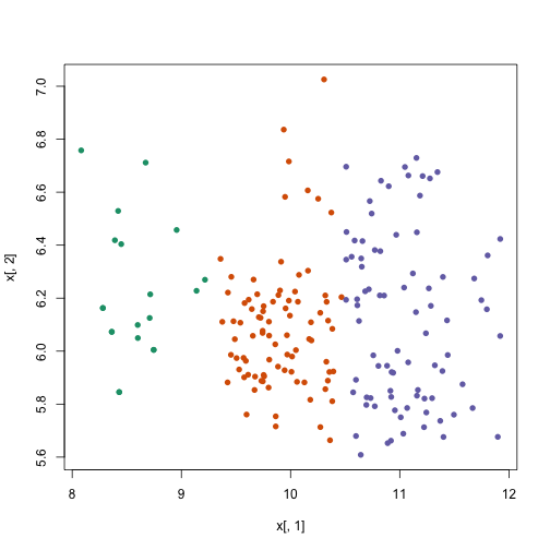
Note that if we perform k-means clustering using all of the genes, the results are not the same as before. Looking at the first two genes doesn’t explain why the clusters we see were generated. So we need to use a different method to see these inter-samples distances.

km <- kmeans(x, centers = 3)
plot(x[, 1], x[, 2], col = km$cluster, pch = 16)

plot of chunk unnamed-chunk-6

Let’s try one last time with larger ‘k’:

km <- kmeans(x, centers = 7)
table(true = t$Tissue, cluster = km$cluster)

##              cluster
## true           1  2  3  4  5  6  7
##   cerebellum   2  0  0  0 19  5 12
##   colon        0 34  0  0  0  0  0
##   endometrium  0  0  0 15  0  0  0
##   hippocampus  0  0  0  0  0 31  0
##   kidney       2  0  0 37  0  0  0
##   liver        2  0 24  0  0  0  0
##   placenta     0  6  0  0  0  0  0