Interactive visualization of DNA methylation data analysis
contributed by Héctor Corrada Bravo
Here we show how to visualize the results of your methylation data analysis in the epiviz interactive
genomics data visualization app. To plot your data there we use the Bioconductor epivizr package.
# biocLite("epivizr")
library(epivizr)
## Loading required package: methods
## Loading required package: Biobase
## Loading required package: BiocGenerics
## Loading required package: parallel
##
## Attaching package: 'BiocGenerics'
##
## The following objects are masked from 'package:parallel':
##
##     clusterApply, clusterApplyLB, clusterCall, clusterEvalQ,
##     clusterExport, clusterMap, parApply, parCapply, parLapply,
##     parLapplyLB, parRapply, parSapply, parSapplyLB
##
## The following object is masked from 'package:stats':
##
##     xtabs
##
## The following objects are masked from 'package:base':
##
##     anyDuplicated, append, as.data.frame, as.vector, cbind,
##     colnames, do.call, duplicated, eval, evalq, Filter, Find, get,
##     intersect, is.unsorted, lapply, Map, mapply, match, mget,
##     order, paste, pmax, pmax.int, pmin, pmin.int, Position, rank,
##     rbind, Reduce, rep.int, rownames, sapply, setdiff, sort,
##     table, tapply, union, unique, unlist
##
## Welcome to Bioconductor
##
##     Vignettes contain introductory material; view with
##     'browseVignettes()'. To cite Bioconductor, see
##     'citation("Biobase")', and for packages 'citation("pkgname")'.
##
## Loading required package: GenomicRanges
## Loading required package: IRanges
## Loading required package: GenomeInfoDb
We assume you already ran the methylation lab. The following code is used to populate the environment with the necessary objects. Please see the methylation lab for description of what these functions are doing.
library(coloncancermeth)
data(coloncancermeth)
library(limma)
##
## Attaching package: 'limma'
##
## The following object is masked from 'package:BiocGenerics':
##
##     plotMA
X<-model.matrix(~pd$Status)
fit<-lmFit(meth,X)
eb <- ebayes(fit)
library(bumphunter)
## Loading required package: foreach
## Loading required package: iterators
## Loading required package: locfit
## locfit 1.5-9.1 	 2013-03-22
chr=as.factor(seqnames(gr))
pos=start(gr)
cl=clusterMaker(chr,pos,maxGap=500)
res<-bumphunter(meth,X,chr=chr,pos=pos,cluster=cl,cutoff=0.1,B=0)
## [bumphunterEngine] Using a single core (backend: doSEQ, version: 1.4.2).
## [bumphunterEngine] Computing coefficients.
## [bumphunterEngine] Finding regions.
## [bumphunterEngine] Found 68682 bumps.
You should therefore have in your environment the following objects:
# the result of using limma and eBayes at the single CpG level
head(fit$coef)
##            (Intercept) pd$Statuscancer
## cg13869341     0.87368      -0.0204296
## cg14008030     0.64920      -0.0098392
## cg12045430     0.05553       0.0560400
## cg20826792     0.19228       0.0243989
## cg00381604     0.01733       0.0008442
## cg20253340     0.54701      -0.0482179
head(eb$t)
##            (Intercept) pd$Statuscancer
## cg13869341      72.059         -1.3625
## cg14008030      46.985         -0.5758
## cg12045430       6.131          5.0036
## cg20826792      20.855          2.1398
## cg00381604       5.167          0.2035
## cg20253340      18.997         -1.3540
# the result of running bumphunter
head(res$fitted)
##                  [,1]
## cg13869341 -0.0204296
## cg14008030 -0.0098392
## cg12045430  0.0560400
## cg20826792  0.0243989
## cg00381604  0.0008442
## cg20253340 -0.0482179
head(res$table)
##        chr     start       end  value  area cluster indexStart indexEnd  L
## 6158  chr6 133561614 133562776 0.4049 16.19   77677     180994   181033 40
## 6568  chr7  27182493  27185282 0.3023 15.42   83616     195992   196042 51
## 5566  chr6  29520698  29521803 0.3798 14.81   71534     158794   158832 39
## 8453 chr10   8094093   8098005 0.2407 14.20  110074     251746   251804 59
## 9015 chr10 118030848 118034357 0.3845 11.53  117242     267198   267227 30
## 5698  chr6  32063774  32064945 0.2798 11.19   72201     165924   165963 40
##      clusterL
## 6158       43
## 6568       53
## 5566       40
## 8453       60
## 9015       30
## 5698       73
# the CpG location object
show(gr)
## GRanges with 485512 ranges and 0 metadata columns:
##              seqnames               ranges strand
##                 <Rle>            <IRanges>  <Rle>
##   cg13869341     chr1       [15865, 15865]      *
##   cg14008030     chr1       [18827, 18827]      *
##   cg12045430     chr1       [29407, 29407]      *
##   cg20826792     chr1       [29425, 29425]      *
##   cg00381604     chr1       [29435, 29435]      *
##          ...      ...                  ...    ...
##   cg17939569     chrY [27009430, 27009430]      *
##   cg13365400     chrY [27210334, 27210334]      *
##   cg21106100     chrY [28555536, 28555536]      *
##   cg08265308     chrY [28555550, 28555550]      *
##   cg14273923     chrY [28555912, 28555912]      *
##   ---
##   seqlengths:
##     chr1  chr2  chr3  chr4  chr5  chr6 ... chr20 chr21 chr22  chrX  chrY
##       NA    NA    NA    NA    NA    NA ...    NA    NA    NA    NA    NA
epivizr uses GRanges objects to visualize data, so we’ll create a new GRanges object containing CpG level
estimates we want to visualize
cpgGR <- gr
cpgGR$fitted <- round(res$fitted,digits=3)
and make another GRanges object containing the bumphunter result
dmrGR <- with(res$table,GRanges(chr,IRanges(start,end),area=area,value=value))

# let's add an annotation for "hypo-" or "hyper-" methylation (as long as the difference is large enough)
dmrGR$type <- ifelse(abs(dmrGR$value)<0.2, "neither", ifelse(dmrGR$value<0,"hypo","hyper"))
table(dmrGR$type)
##
##   hyper    hypo neither
##    5141   18865   44676
Now, we are ready to visualize this data on epiviz. First start an epiviz session:
mgr <- startEpiviz(workspace="mi9NojjqT1l")
## [epivizr] Starting websocket server...
Windows users You need to call the mgr$service() method to allow the epiviz app to connect to your R session:
# mgr$service()
Non-Windows users don’t need to do this.
Now, let’s add tracks for hypo and hyper methylated regions:
hypoTrack <- mgr$addDevice(subset(dmrGR,dmrGR$type=="hypo"), "Hypo-methylated")
hyperTrack <- mgr$addDevice(subset(dmrGR,dmrGR$type=="hyper"), "Hyper-methylated")
We can also add the estimated methylation difference as another track:
diffTrack <- mgr$addDevice(cpgGR,"Meth difference",type="bp",columns="fitted")
Go to your browser and navigate around, search for your favorite gene and take a look at gene expression
looks like around these regions according to the gene expression barcode,
which we preloaded when we started epiviz. Here’s some interesting ones: “MMP10”, “TIMP2”, “MAGEA12”.
<img src=”figure/epiviz.png” width=600 />
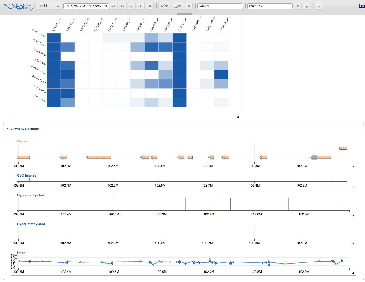
Windows users Remember to call mgr$service() before going to the browser
Here’s other useful analyses you can do with epivizr. Let’s make a SummarizedExperiment containing CpG-level data we can use for an MA plot
colData <- DataFrame(name=c("M","A"))
rownames(colData) <- colData$name

rowData <- gr
rowData$cpg <- names(gr)

cpgSE <- SummarizedExperiment(rowData=rowData,
      assays=SimpleList(ma=cbind(fit$coef[,2],fit$Amean)),
      colData=colData)
and add the MA plot:
maPlot <- mgr$addDevice(cpgSE,columns=c("A","M"),"cpg MA")
<img src=”figure/epivizma.png” width=600 />
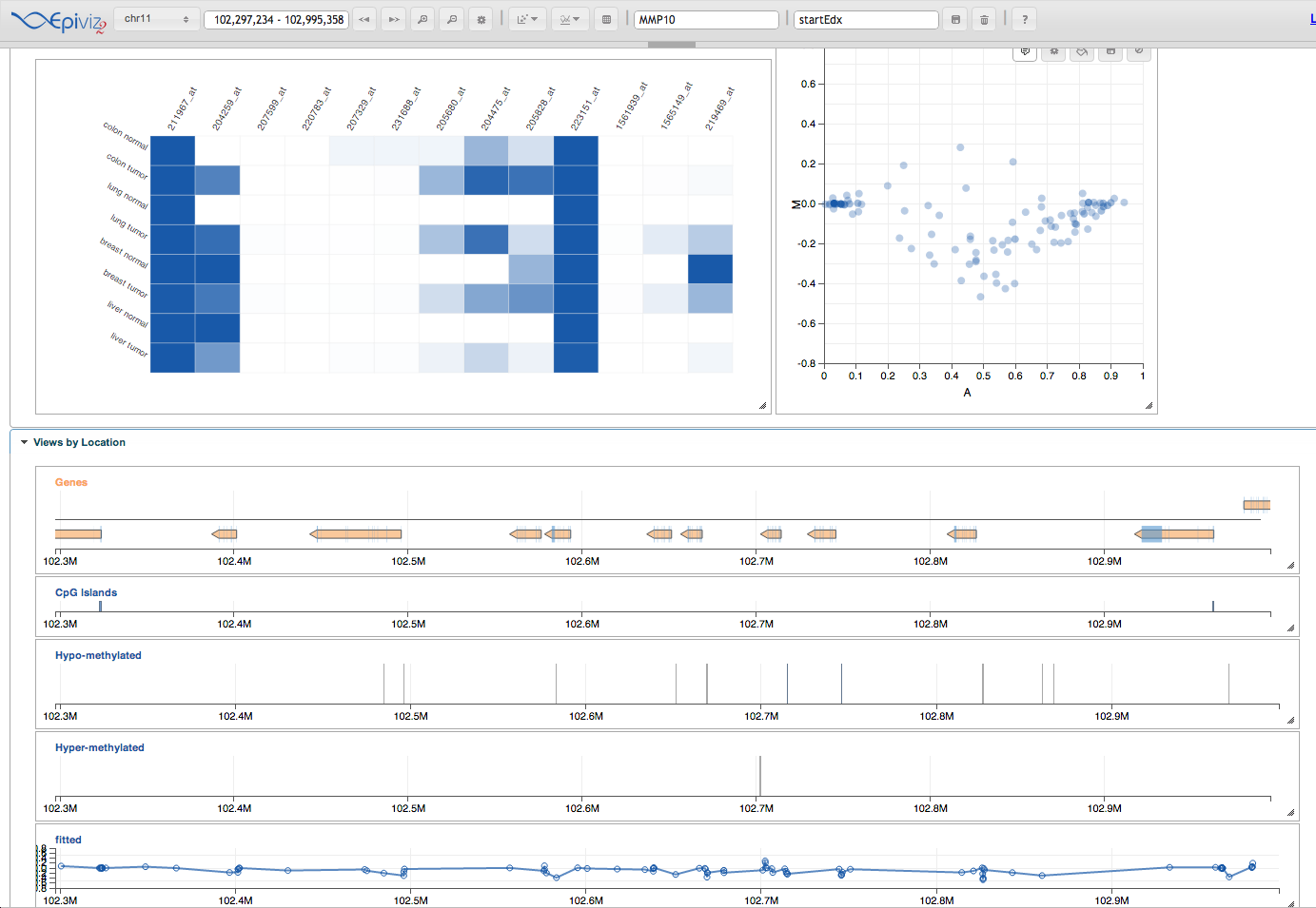
Let’s now browse the genome in order through the top 5 found regions in order (by area):
slideshowRegions <- dmrGR[1:10,] + 10000
mgr$slideshow(slideshowRegions, n=5)
## Region 1 of 5 . Press key to continue (ESC to stop)...
## Region 2 of 5 . Press key to continue (ESC to stop)...
## Region 3 of 5 . Press key to continue (ESC to stop)...
## Region 4 of 5 . Press key to continue (ESC to stop)...
## Region 5 of 5 . Press key to continue (ESC to stop)...
Last thing to do is disconnect the epiviz app:
mgr$stopServer()
There’s a lot more you can do with epiviz. It’s a fairly flexible visualization tool. You can find out more about it in the epiviz documentation site.
Also, epivizr has a vignette that’s worth checking out:
browseVignettes("epivizr")
## starting httpd help server ... done