Introduction

We introduce EDA for univariate data. Here we describe EDA and summary statistics for paired data.

Scatterplots and correlation

The methods described above relate to univariate variables. In the biomedical sciences it is common to be interested in the relationship between two or more variables. A classic examples is the father/son height data used by Galton to understand heredity. Were we to summarize these data we could use the two averages and two standard deviations as both distributions are well approximated by the normal distribution. This summary, however, fails to describe an important characteristic of the data.

# install.packages("UsingR")
library(UsingR)

## Loading required package: MASS
## Loading required package: HistData
## Loading required package: Hmisc
## Loading required package: methods
## Loading required package: grid
## Loading required package: lattice
## Loading required package: survival
## Loading required package: splines
## Loading required package: Formula
## 
## Attaching package: 'Hmisc'
## 
## The following objects are masked from 'package:base':
## 
##     format.pval, round.POSIXt, trunc.POSIXt, units
## 
## 
## Attaching package: 'UsingR'
## 
## The following object is masked from 'package:survival':
## 
##     cancer

data("father.son")
x=father.son$fheight
y=father.son$sheight
plot(x,y,xlab="Father's height in inches",ylab="Son's height in inches",main=paste("correlation =",signif(cor(x,y),2)))

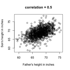
The scatter plot shows a general trend: the taller the father the taller to son. A summary of this trend is the correlation coefficient which in this cases is 0.5. We motivate this statistic by trying to predict son’s height using the father’s.

Stratification

Suppose we are asked to guess the height of randomly select sons. The average height, 68.7 inches, is the value with the highest proportion (see histogram) and would be our prediction. But what if we are told that the father is 72 inches tall, do we sill guess 68.7?

Note that the father is taller than average. He is 1.7 standard deviations taller than the average father. So should we predict that the son is also 1.75 standard deviations taller? Turns out this is an overestimate. To see this we look at all the sons with fathers who are about 72 inches. We do this by stratifying the son heights.

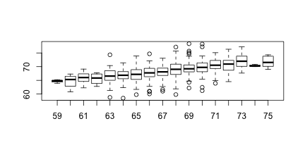
groups <- split(y,round(x)) 
boxplot(groups)

print(mean(y[ round(x) == 72]))

## [1] 70.67719

Stratification followed by boxplots lets us see the distribution of each group. The average height of sons with fathers that are 72 is 70.7. We also see that the means of the strata appear to follow a straight line. This line is refereed to the regression line and it’s slope is related to the correlation.

Bi-variate normal distribution

A pair of random variable $(X,y)$ is considered to be approximated by bivariate normal when the proportion of values below, say $x$ and $y$ is approximated by this expression:

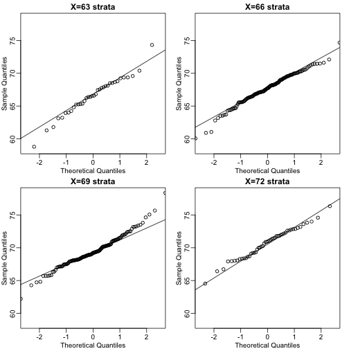
A definition that is more intuitive is the following. Fix a value $x$ and look at all the pairs $(X,Y)$ for which $X=x$. Generally, in Statistics we call this exercise conditionion. We are conditioning $Y$ on $X$. If a pair of random variables is approximated by a bivariate normal distribution then the distribution of $Y$ condition on $X=x$ is approximated with a normal distribution for all $x$. Let’s see if this happens here. We take 4 different strata to demonstrate this:

groups <- split(y,round(x)) 
mypar2(2,2)
for(i in c(5,8,11,14)){
  qqnorm(groups[[i]],main=paste0("X=",names(groups)[i]," strata"),
         ylim=range(y),xlim=c(-2.5,2.5))
  qqline(groups[[i]])
}

Now we come back to defining correlation. Mathematical statistics tells us that when two variables follow a bivariate normal distribution then for any given value of $x$ the average of the $Y$ in pairs for which $X=x$ is

Note that this is a line with slope $r \frac{\sigma_Y}{\sigma_X}$. This is referred to as the regression line. Note also that if the SDs are the same, then the slope of the regression line is the correlation $r$. Therefore, if we standardize $X$ and $Y$ the correlation is the slope of the regression line.

Another way to see this is that to form a prediction $\hat{Y}$, for every SD away from the mean in $x$, we predict $r$ SDs away for $Y$:

with the $\mu$ representing the averages, $\sigma$ the standard deviations, and $r$ the correlation. So if there is perfect correlation we predict the same number of SDs, if there is 0 correlation then we don’t use $x$ at all, and for values between 0 and 1, the prediction is somewhere in between. For negative values, we simply predict in the opposite direction.

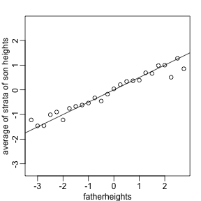
To confirm that the above approximations hold here, let’s compare the mean of each strata to the identity line and the regression line

x=(x-mean(x))/sd(x)
y=(y-mean(y))/sd(y)
means=tapply(y,round(x*4)/4,mean)
fatherheights=as.numeric(names(means))
mypar2(1,1)
plot(fatherheights,means,ylab="average of strata of son heights",ylim=range(fatherheights))
abline(0,cor(x,y))

Spearman’s correlation

Just like the average and standard deviation are not good summaries when the data is not well approximated by the normal distribution, the correlation is not a good summary when pairs of lists are not approximated by the bivariate normal distribution. Examples include cases in which on variable is related to another by a parabolic function. Another, more common example are caused by outliers or extreme values.

a=rnorm(100);a[1]=10
b=rnorm(100);b[1]=11
plot(a,b,main=paste("correlation =",signif(cor(a,b),2)))

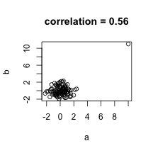In the example above the data are not associated but for one pair both values are very large. The correlation here is about 0.5. This is driven by just that one point as taking it out lowers to correlation to about 0. An alternative summary for cases with outliers or extreme values is Spearman’s correlation which is based on ranks instead of the values themselves.