Hierarchical Models

In this section, we use the mathematical theory which describes an approach that has become widely applied in the analysis of high-throughput data. The general idea is to build a hierachichal model with two levels. One level describes variability across samples/units, and the other describes variability across features. This is similar to the baseball example in which the first level described variability across players and the second described the randomness for the success of one player. The first level of variation is accounted for by all the models and approaches we have described here, for example the model that leads to the t-test. The second level provides power by permitting us to “borrow” information from all features to inform the inference performed on each one.

Here we describe one specific case that is currently the most widely used approach to inference with gene expression data. It is the model implemented by the limma Bioconductor package. This idea has been adapted to develop methods for other data types such as RNAseq by, for example, edgeR and DESeq2. This package provides an alternative to the t-test that greatly improves power by modeling the variance. While in the baseball example we modeled averages, here we model variances. Modelling variances requires more advanced math, but the concepts are practically the same. We motivate and demonstrate the approach with an example.

Here is a volcano showing effect sizes and p-value from applying a t-test to data from an experiment running six replicated samples with 16 genes artificially made to be different in two groups of three samples each. These 16 genes are the only genes for which the alternative hypothesis is true. In the plot they are shown in blue.

library(SpikeInSubset) ##Available from Bioconductor
data(rma95)
library(genefilter)
fac <- factor(rep(1:2,each=3))
tt <- rowttests(exprs(rma95),fac)
smallp <- with(tt, p.value < .01)
spike <- rownames(rma95) %in% colnames(pData(rma95))
cols <- ifelse(spike,"dodgerblue",ifelse(smallp,"red","black"))

with(tt, plot(-dm, -log10(p.value), cex=.8, pch=16,
     xlim=c(-1,1), ylim=c(0,4.5),
     xlab="difference in means",
     col=cols))
abline(h=2,v=c(-.2,.2), lty=2)

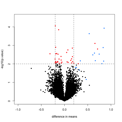
We cut-off the range of the y-axis at 4.5, but there is one blue point with a p-value smaller than $10^{-6}$. Two findings stand out from this plot. The first is that only one of the positives would be found to be significant with a standard 5% FDR cutoff:

sum( p.adjust(tt$p.value,method = "BH")[spike] < 0.05)

## [1] 1

This of course has to do with the low power associated with a sample size of three in each group. The second finding is that if we forget about inference and simply rank the genes based on the size of the t-statistic, we obtain many false positives in any rank list of size larger than 1. For example, six of the top 10 genes ranked by t-statistic are false positives.

table( top50=rank(tt$p.value)<= 10, spike) #t-stat and p-val rank is the same

##        spike
## top50   FALSE  TRUE
##   FALSE 12604    12
##   TRUE      6     4

In the plot we notice that these are mostly genes for which the effect size is relatively small, implying that the estimated standard error is small. We can confirm this with a plot:

tt$s <- apply(exprs(rma95), 1, function(row) 
  sqrt(.5 * (var(row[1:3]) + var(row[4:6]) ) ) )
with(tt, plot(s, -log10(p.value), cex=.8, pch=16,
              log="x",xlab="estimate of standard deviation",
              col=cols))

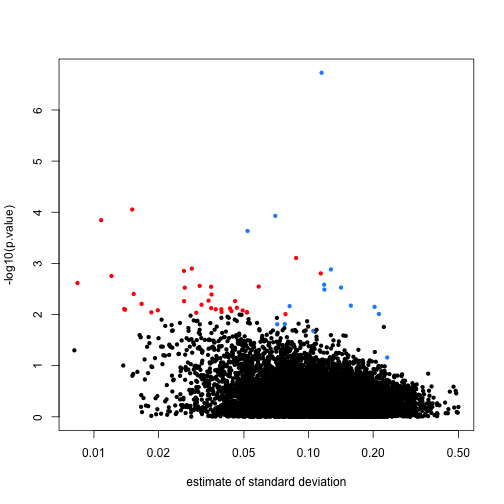
Here is where a hierarchical model can be useful. If we can make an assumption about the distribution of these variances across genes, then we can improve estimates by “adjusting” estimates that are “too small” according to this distribution. In a previous section we described how the F-distribution approximates the distribution of the observed variances.

Because we have thousands of data points, we can actually check this assumption and also estimate the parameters $s_0$ and $d_0$. This particular approach is referred to as empirical Bayes because it can be described as using data (empirical) to build the prior distribution (Bayesian approach).

Now we apply what we learned with the baseball example to the standard error estimates. As before we have an observed value for each gene $s_g$, a sampling distribution as a prior distribution. We can therefore compute a posterior distribution for the variance $\sigma^2_g$ and obtain the posterior mean. You can see the details of the derivation in this paper.

As in the baseball example, the posterior mean shrinks the observed variance $s_g^2$ towards the global variance $s_0^2$ and the weights depend on the sample size through the degrees of freedom $d$ and, in this case, the shape of the prior distribution through $d_0$.

In the plot above we can see how the variance estimate shrink for 40 genes (code not shown):

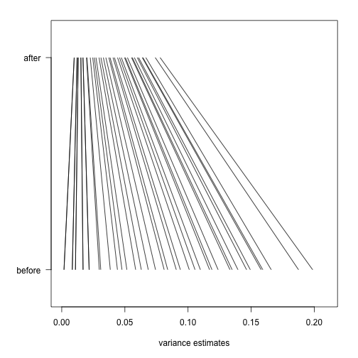
An important aspect of this adjustment is that genes having a sample standard deviation close to 0 are no longer close to 0 (the shrink towards $s_0$ ). We can now create a version of the t-test that instead of the sample standard deviation uses this posterior mean or “shrunken” estimate of the variance. We refer to these as moderated t-tests. Once we do this, the improvements can be seen clearly in the volcano plot:

library(limma)
fit <- lmFit(rma95, model.matrix(~ fac))
ebfit <- ebayes(fit)
limmares <- data.frame(dm=coef(fit)[,"fac2"], p.value=ebfit$p.value[,"fac2"])
with(limmares, plot(dm, -log10(p.value),cex=.8, pch=16,
     col=cols,xlab="difference in means",
     xlim=c(-1,1), ylim=c(0,5)))
abline(h=2,v=c(-.2,.2), lty=2)

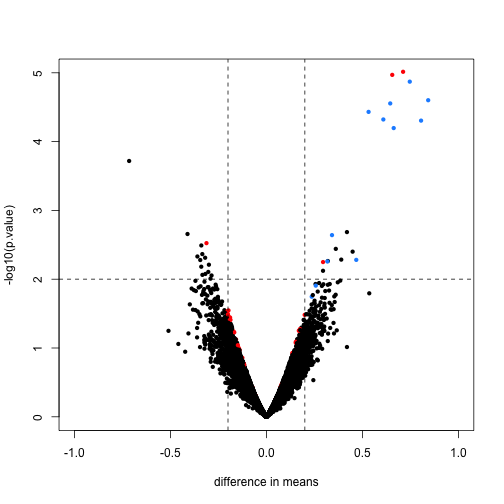
The number of false positives in the top 10 is now reduced to 2.

table( top50=rank(limmares$p.value)<= 10, spike) 

##        spike
## top50   FALSE  TRUE
##   FALSE 12608     8
##   TRUE      2     8