Inference in Practice

Suppose we were given high-throughput gene expression data that was measured for several individuals in two populations. We are asked to report which genes have different average expression levels in the two populations. If instead of thousands of genes, we were handed data from just one gene, we could simply apply the inference techniques that we have learned before. We could, for example, use a t-test or some other test. Here we review what changes when we consider high-throughput data.

p-values are random variables

An important concept to remember in order to understand the concepts presented in this chapter is that p-values are random variables. To see this, consider the example in which we define a p-value from a t-test with a large enough sample size to use the CLT approximation. Then our p-value is defined as the probability that a normally distributed random variable is larger, in absolute value, than the observed t-test, call it $Z$. So for a two sided test the p-value is:

In R, we write:

2*(1-pnorm(Z))

Now because $Z$ is a random variable and $\Phi$ is a deterministic function, $p$ is also a random variable. We will create a Monte Carlo simulation showing how the values of $p$ change. We use femaleControlsPopulation.csv from earlier chapters.

We read in the data, and use replicate to repeatedly create p-values.

set.seed(1)
population = unlist( read.csv("femaleControlsPopulation.csv") )
N <- 12
B <- 10000
pvals <- replicate(B,{
  control = sample(population,N)
  treatment = sample(population,N)
  t.test(treatment,control)$p.val 
  })
hist(pvals)

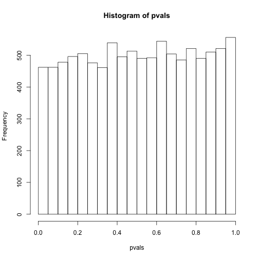
As implied by the histogram, in this case the distribution of the p-value is uniformly distributed. In fact, we can show theoretically that when the null hypothesis is true, this is always the case. For the case in which we use the CLT, we have that the null hypothesis $H_0$ implies that our test statistic $Z$ follows a normal distribution with mean 0 and SD 1 thus:

This implies that:

which is the definition of a uniform distribution.

Thousands of tests

In this data we have two groups denoted with 0 and 1:

library(GSE5859Subset)
data(GSE5859Subset)
g <- sampleInfo$group
g

##  [1] 1 1 1 1 1 1 1 1 1 1 1 1 0 0 0 0 0 0 0 0 0 0 0 0

If we were interested in a particular gene, let’s arbitrarily pick the one on the 25th row, we would simply compute a t-test. To compute a p-value, we will use the t-distribution approximation and therefore we need the population data to be approximately normal. We check this assumption with a qq-plot:

e <- geneExpression[25,]

library(rafalib)
mypar(1,2)

qqnorm(e[g==1])
qqline(e[g==1])

qqnorm(e[g==0])
qqline(e[g==0])

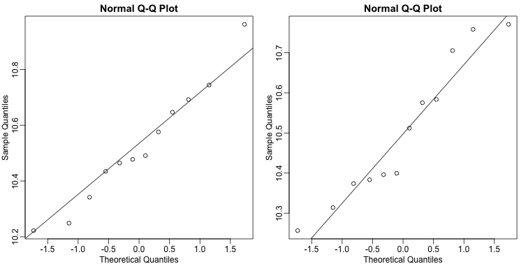
The qq-plots show that the data is well approximated by the normal approximation. The t-test does not find this gene to be statistically significant:

t.test(e[g==1],e[g==0])$p.value

## [1] 0.779303

To answer the question for each gene, we simply do repeat the above for each gene. Here we will define our own function and use apply:

myttest <- function(x) t.test(x[g==1],x[g==0],var.equal=TRUE)$p.value
pvals <- apply(geneExpression,1,myttest)

We can now see which genes have p-values less than, say, 0.05. For example, right away we see that…

sum(pvals<0.05)

## [1] 1383

… genes had p-values less than 0.05.

However, as we will describe in more detail below, we have to be careful in interpreting this result because we have performed over 8,000 tests. If we performed the same procedure on random data, for which the null hypothesis is true for all features, we obtain the following results:

set.seed(1)
m <- nrow(geneExpression)
n <- ncol(geneExpression)
randomData <- matrix(rnorm(n*m),m,n)
nullpvals <- apply(randomData,1,myttest)
sum(nullpvals<0.05)

## [1] 419

As we will explain later in the chapter, this is to be expected: 419 is roughly 0.05*8192 and we will describe the theory that tells us why this prediction works.

Faster t-test implementation

Before we continue, we should point out that the above implementation is very inefficient. There are several faster implementations that perform t-test for high-throughput data. We make use of a function that is not available from CRAN, but rather from the Bioconductor project.

To download and install packages from Bioconductor, we can use the install_bioc function in rafalib to install the package:

install_bioc("genefilter")

Now we can show that this function is much faster than our code above and produce practically the same answer:

library(genefilter)
results <- rowttests(geneExpression,factor(g))
max(abs(pvals-results$p))

## [1] 6.528111e-14