Monte Carlo Simulation

Computers can be used to generate pseudo-random numbers. For practical purposes these pseudo-random numbers can be used to imitate random variables from the real world. This permits us to examine properties of random variables using a computer instead of theoretical or analytical derivations. One very useful aspect of this concept is that we can create simulated data to test out ideas or competing methods, without actually having to perform laboratory experiments.

Simulations can also be used to check theoretical or analytical results. Also, many of the theoretical results we use in statistics are based on asymptotics: they hold when the sample size goes to infinity. In practice, we never have an infinite number of samples so we may want to know how well the theory works with our actual sample size. Sometimes we can answer this question analytically, but not always. Simulations are extremely useful in these cases.

As an example, let’s use a Monte Carlo simulation to compare the CLT to the t-distribution approximation for different sample sizes.

library(dplyr)
dat <- read.csv("mice_pheno.csv")
controlPopulation <- filter(dat,Sex == "F" & Diet == "chow") %>%  
  select(Bodyweight) %>% unlist

We will build a function that automatically generates a t-statistic under the null hypothesis for a any sample size of n.

ttestgenerator <- function(n) {
  #note that here we have a false "high fat" group where we actually
  #sample from the nonsmokers. this is because we are modeling the *null*
  cases <- sample(controlPopulation,n)
  controls <- sample(controlPopulation,n)
  tstat <- (mean(cases)-mean(controls)) / 
      sqrt( var(cases)/n + var(controls)/n ) 
  return(tstat)
  }
ttests <- replicate(1000, ttestgenerator(10))

With 1,000 Monte Carlo simulated occurrences of this random variable, we can now get a glimpse of its distribution:

hist(ttests)

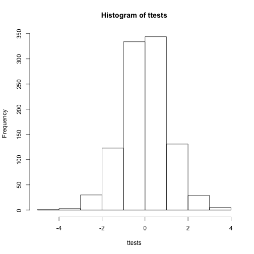
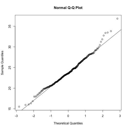
So is the distribution of this t-statistic well approximated by the normal distribution? In the next chapter, we will formally introduce quantile-quantile plots, which provide a useful visual inspection of how well one distribution approximates another. As we will explain later, if points fall on the identity line, it means the approximation is a good one.

qqnorm(ttests)
abline(0,1)

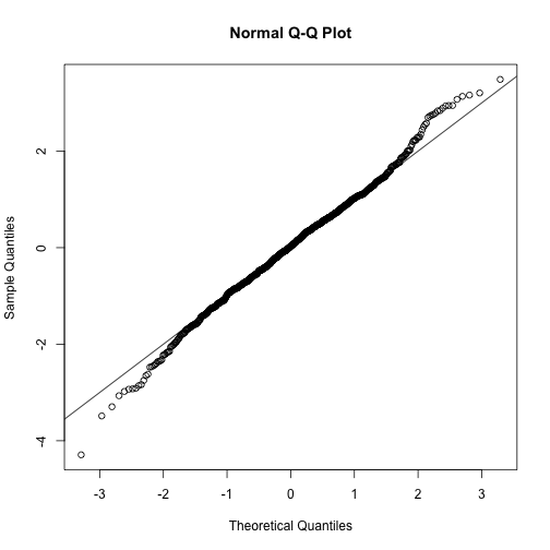
This looks like a very good approximation. For this particular population, a sample size of 10 was large enough to use the CLT approximation. How about 3?

ttests <- replicate(1000, ttestgenerator(3))
qqnorm(ttests)
abline(0,1)

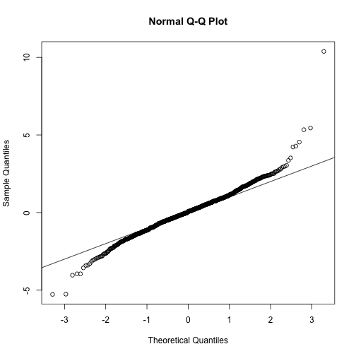
Now we see that the large quantiles, referred to by statisticians as the tails, are larger than expected (below the line on the left side of the plot and above the line on the right side of the plot). In the previous module, we explained that when the sample size is not large enough and the population values follow a normal distribution, then the t-distribution is a better approximation. Our simulation results seem to confirm this:

ps <- (seq(0,999)+0.5)/1000
qqplot(qt(ps,df=2*3-2),ttests,xlim=c(-6,6),ylim=c(-6,6))
abline(0,1)

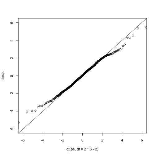
The t-distribution is a much better approximation in this case, but it is still not perfect. This is due to the fact that the original data is not that well approximated by the normal distribution.

qqnorm(controlPopulation)
qqline(controlPopulation)

Parametric Simulations for the Observations

The technique we used to motivate random variables and the null distribution was a type of Monte Carlo simulation. We had access to population data and generated samples at random. In practice, we do not have access to the entire population. The reason for using the approach here was for educational purposes. However, when we want to use Monte Carlo simulations in practice, it is much more typical to assume a parametric distribution and generate a population from this, which is called a parametric simulation. This means that we take parameters estimated from the real data (here the mean and the standard deviation), and plug these into a model (here the normal distribution). This is actually the most common form of Monte Carlo simulation.

For the case of weights, we could use our knowledge that mice typically weigh 24 ounces with a SD of about 3.5 ounces, and that the distribution is approximately normal, to generate population data:

controls<- rnorm(5000, mean=24, sd=3.5) 

After we generate the data, we can then repeat the exercise above. We no longer have to use the sample function since we can re-generate random normal numbers. The ttestgenerator function therefore can be written as follows:

ttestgenerator <- function(n, mean=24, sd=3.5) {
  cases <- rnorm(n,mean,sd)
  controls <- rnorm(n,mean,sd)
  tstat <- (mean(cases)-mean(controls)) / 
      sqrt( var(cases)/n + var(controls)/n ) 
  return(tstat)
  }