Projections

Now that we have described the concept of dimension reduction and some of the applications of SVD and principal component analysis, we focus on more details related to the mathematics behind these. We start with projections. A projection is a linear algebra concept that helps us understand many of the mathematical operations we perform on high-dimensional data. For more details, you can review projects in a linear algebra book. Here we provide a quick review and then provide some data analysis related examples.

As a review, remember that projections minimize the distance between points and subspace.

In the figure above, the point on top is pointing to a point in space. In this particular cartoon, the space is two dimensional, but we should be thinking abstractly. The space is represented by the Cartesian plan and the line on which the little person stands is a subspace of points. The projection to this subspace is the place that is closest to the original point. Geometry tells us that we can find this closest point by dropping a perpendicular line (dotted line) from the point to the space. The little person is standing on the projection. The amount this person had to walk from the origin to the new projected point is referred to as the coordinate.

For the explanation of projections, we will use the standard matrix algebra notation for points: $\vec{y} \in \mathbb{R}^N$ is a point in $N$-dimensional space and $L \subset \mathbb{R}^N$ is smaller subspace.

Simple example with N=2

If we let $Y = \begin{pmatrix} 2 \\ 3\end{pmatrix}$. We can plot it like this:

mypar (1,1)
plot(c(0,4),c(0,4),xlab="Dimension 1",ylab="Dimension 2",type="n")
arrows(0,0,2,3,lwd=3)
text(2,3," Y",pos=4,cex=3)

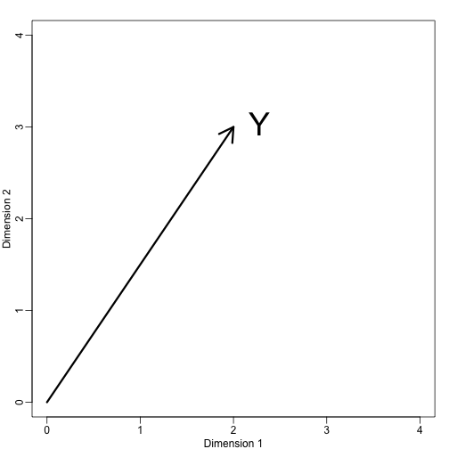
We can immediately define a coordinate system by projecting this vector to the space defined by: $\begin{pmatrix} 1\\ 0\end{pmatrix}$ (the x-axis) and $\begin{pmatrix} 0\\ 1\end{pmatrix}$ (the y-axis). The projections of $Y$ to the subspace defined by these points are 2 and 3 respectively:

We say that $2$ and $3$ are the coordinates and that $\begin{pmatrix} 1\\ 0\end{pmatrix} \mbox{and} \begin{pmatrix} 0\\1 \end{pmatrix}$ are the bases.

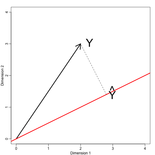
Now let’s define a new subspace. The red line in the plot below is subset $L$ defined by points satisfying $c \vec{v}$ with $\vec{v}=\begin{pmatrix} 2& 1\end{pmatrix}^\top$. The projection of $\vec{y}$ onto $L$ is the closest point on $L$ to $\vec{y}$. So we need to find the $c$ that minimizes the distance between $\vec{y}$ and $c\vec{v}=(2c,c)$. In linear algebra, we learn that the difference between these points is orthogonal to the space so:

this implies that:

and:

Here the dot $\cdot$ represents the dot product: $\,\, \vec{x} \cdot \vec{y} = x_1 y_1+\dots x_n y_n$.

The following R code confirms this equation works:

mypar(1,1)
plot(c(0,4),c(0,4),xlab="Dimension 1",ylab="Dimension 2",type="n")
arrows(0,0,2,3,lwd=3)
abline(0,0.5,col="red",lwd=3) #if x=2c and y=c then slope is 0.5 (y=0.5x)
text(2,3," Y",pos=4,cex=3)
y=c(2,3)
x=c(2,1)
cc = crossprod(x,y)/crossprod(x)
segments(x[1]*cc,x[2]*cc,y[1],y[2],lty=2)
text(x[1]*cc,x[2]*cc,expression(hat(Y)),pos=4,cex=3)

Note that if $\vec{v}$ was such that $\vec{v}\cdot \vec{v}=1$, then $\hat{c}$ is simply $\vec{y} \cdot \vec{v}$ and the space $L$ does not change. This simplification is one reason we like orthogonal matrices.

Example: The sample mean is a projection

Let $\vec{y} \in \mathbb{R}^N$ and $L \subset \mathbb{R}^N$ is the space spanned by:

In this space, all components of the vectors are the same number, so we can think of this space as representing the constants: in the projection each dimension will be the same value. So what $c$ minimizes the distance between $c\vec{v}$ and $\vec{y}$ ?

When talking about problems like this, we sometimes use 2 dimensional figures such as the one above. We simply abstract and think of $\vec{y}$ as a point in $N-dimensions$ and $L$ as a subspace defined by a smaller number of values, in this case just one: $c$.

Getting back to our question, we know that the projection is:

which in this case is the average:

Here, it also would have been just as easy to use calculus:

Example: Regression is also a projection

Let us give a slightly more complicated example. Simple linear regression can also be explained with projections. Our data $\mathbf{Y}$ (we are no longer going to use the $\vec{y}$ notation) is again an $N-dimensional$ vector and our model predicts $Y_i$ with a line $\beta_0 + \beta_1 X_i$. We want to find the $\beta_0$ and $\beta_1$ that minimize the distance between $Y$ and the space defined by:

with:

Our $N\times 2$ matrix $\mathbf{X}$ is $[ \vec{v}_0 \,\, \vec{v}_1]$ and any point in $L$ can be written as $X\vec{\beta}$.

The equation for the multidimensional version of orthogonal projection is:

which we have seen before and gives us:

And the projection to $L$ is therefore: