Principal Component Analysis

We have already mentioned principal component analysis (PCA) above and noted its relation to the SVD. Here we provide further mathematical details.

Example: Twin heights

We started the motivation for dimension reduction with a simulated example and showed a rotation that is very much related to PCA.

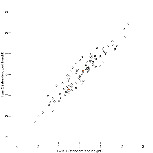
Here we explain specifically what are the principal components (PCs).

Let $\mathbf{Y}$ be $2 \times N$ matrix representing our data. The analogy is that we measure expression from 2 genes and each column is a sample. Suppose we are given the task of finding a $2 \times 1$ vector $\mathbf{u}_1$ such that $\mathbf{u}_1^\top \mathbf{v}_1 = 1$ and it maximizes $(\mathbf{u}_1^\top\mathbf{Y})^\top (\mathbf{u}_1^\top\mathbf{Y})$. This can be viewed as a projection of each sample or column of $\mathbf{Y}$ into the subspace spanned by $\mathbf{u}_1$. So we are looking for a transformation in which the coordinates show high variability.

Let’s try $\mathbf{u}=(1,0)^\top$. This projection simply gives us the height of twin 1 shown in orange below. The sum of squares is shown in the title.

mypar(1,1)
plot(t(Y), xlim=thelim, ylim=thelim,
     main=paste("Sum of squares :",round(crossprod(Y[,1]),1)))
abline(h=0)
apply(Y,2,function(y) segments(y[1],0,y[1],y[2],lty=2))

## NULL

points(Y[1,],rep(0,ncol(Y)),col=2,pch=16,cex=0.75)

Can we find a direction with higher variability? How about:

$\mathbf{u} =\begin{pmatrix}1\\-1\end{pmatrix}$ ? This does not satisfy $\mathbf{u}^\top\mathbf{u}= 1$ so let’s instead try $\mathbf{u} =\begin{pmatrix}1/\sqrt{2}\\-1/\sqrt{2}\end{pmatrix}$

u <- matrix(c(1,-1)/sqrt(2),ncol=1)
w=t(u)%*%Y
mypar(1,1)
plot(t(Y),
     main=paste("Sum of squares:",round(tcrossprod(w),1)),xlim=thelim,ylim=thelim)
abline(h=0,lty=2)
abline(v=0,lty=2)
abline(0,-1,col=2)
Z = u%*%w
for(i in seq(along=w))
  segments(Z[1,i],Z[2,i],Y[1,i],Y[2,i],lty=2)
points(t(Z), col=2, pch=16, cex=0.5)

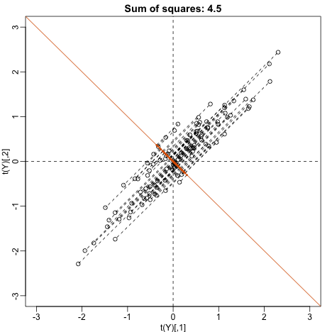
This relates to the difference between twins, which we know is small. The sum of squares confirms this.

Finally, let’s try:

u <- matrix(c(1,1)/sqrt(2),ncol=1)
w=t(u)%*%Y
mypar()
plot(t(Y), main=paste("Sum of squares:",round(tcrossprod(w),1)),
     xlim=thelim, ylim=thelim)
abline(h=0,lty=2)
abline(v=0,lty=2)
abline(0,1,col=2)
points(u%*%w, col=2, pch=16, cex=1)
Z = u%*%w
for(i in seq(along=w))
  segments(Z[1,i], Z[2,i], Y[1,i], Y[2,i], lty=2)
points(t(Z),col=2,pch=16,cex=0.5)

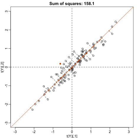
This is a re-scaled average height, which has higher sum of squares. There is a mathematical procedure for determining which $\mathbf{v}$ maximizes the sum of squares and the SVD provides it for us.

The principal components

The orthogonal vector that maximizes the sum of squares:

$\mathbf{u}_1^\top\mathbf{Y}$ is referred to as the first PC. The weights $\mathbf{u}$ used to obtain this PC are referred to as the loadings. Using the language of rotations, it is also referred to as the direction of the first PC, which are the new coordinates.

To obtain the second PC, we repeat the exercise above, but for the residuals:

The second PC is the vector with the following properties:

and maximizes $(\mathbf{rv}_2)^\top \mathbf{rv}_2$.

When $Y$ is $N \times m$ we repeat to find 3rd, 4th, …, m-th PCs.

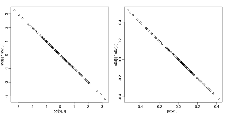
prcomp

We have shown how to obtain PCs using the SVD. However, R has a function specifically designed to find the principal components. In this case, the data is centered by default. The following function:

pc <- prcomp( t(Y) )

produces the same results as the SVD up to arbitrary sign flips:

s <- svd( Y - rowMeans(Y) )
mypar(1,2)
for(i in 1:nrow(Y) ){
  plot(pc$x[,i], s$d[i]*s$v[,i])
}

The loadings can be found this way:

pc$rotation

##            PC1        PC2
## [1,] 0.7072304  0.7069831
## [2,] 0.7069831 -0.7072304

which are equivalent (up to a sign flip) to:

s$u

##            [,1]       [,2]
## [1,] -0.7072304 -0.7069831
## [2,] -0.7069831  0.7072304

The equivalent of the variance explained is included in the:

pc$sdev

## [1] 1.2542672 0.2141882

component.

We take the transpose of Y because prcomp assumes the previously discussed ordering: units/samples in row and features in columns.