Bayesian Statistics

One distinguishing characteristic of high-throughput data is that although we want to report on specific features, we observe many related outcomes. For example, we measure the expression of thousands of genes, or the height of thousands of peaks representing protein binding, or the methylation levels across several CpGs. However, most of the statistical inference approaches we have shown here treat each feature independently and pretty much ignores data from other features. We will learn how using statistical models provides power by modeling features jointly. The most successful of these approaches are what we refer to as hierarchical models, which we explain below in the context of Bayesian statistics.

Bayes theorem

We start by reviewing Bayes theorem. We do this using a hypothetical cystic fibrosis test as an example. Suppose a test for cystic fibrosis has an accuracy of 99%. We will use the following notation:

$\mbox{Prob}(+ \mid D=1)=0.99, \mbox{Prob}(- \mid D=0)=0.99$

with $+$ meaning a positive test and $D$ representing if you actually have the disease (1) or not (0).

Suppose we select a random person and they test positive, what is the probability that they have the disease? We write this as $\mbox{Prob}(D=1 \mid +)?$ The cystic fibrosis rate is 1 in 3,900 which implies that $\mbox{Prob}(D=1)=0.0025$ . To answer this question we will use Bayes Theorem, which in general tells us that:

$\mbox{Pr}(A \mid B) = \frac{\mbox{Pr}(B \mid A)\mbox{Pr}(A)}{\mbox{Pr}(B)}$

This equation applied to our problem becomes:

$\begin{align*} \mbox{Prob}(D=1 \mid +) & = \frac{ P(+ \mid D=1) \cdot P(D=1)} {\mbox{Prob}(+)} \\ & = \frac{\mbox{Prob}(+ \mid D=1)\cdot P(D=1)} {\mbox{Prob}(+ \mid D=1) \cdot P(D=1) + \mbox{Prob}(+ \mid D=0) \mbox{Prob}( D=0)} \end{align*}$

Plugging in the numbers we get:

$\frac{0.99 \cdot 0.0025}{0.99 \cdot 0.0025 + 0.01 \cdot (.9975)} = 0.02$

This says that despite the test having 0.99 accuracy, the probability of having the disease given a positive test is only 0.02. This may appear counterintuitive to some. The reason this is the case is because we have to factor in the very rare probability that a person, chosen at random, has the disease. To illustrate this we run a Monte Carlo simulation.

Simulation

The following simulation is meant to help you visualize Bayes Theorem. We start by randomly selecting 1500 people from a population in which the disease in question has a 5% prevalence.

set.seed(3)
prev <- 1/20
##Later, we are arranging 1000 people in 80 rows and 20 columns
M <- 50 ; N <- 30
##do they have the disease?
d<-rbinom(N*M,1,p=prev)

Now each person gets the test which is correct 90% of the time.

accuracy <- 0.9
test <- rep(NA,N*M)
##do controls test positive?
test[d==1]  <- rbinom(sum(d==1), 1, p=accuracy)
##do cases test positive?
test[d==0]  <- rbinom(sum(d==0), 1, p=1-accuracy)

Because there are so many more controls than cases, even with a low false positive rate, we get more controls than cases in the group that tested positive (code not shown):

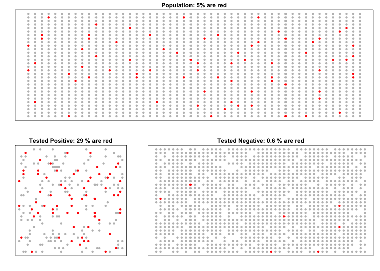
Simulation demonstrating Bayes theorem. Top plot shows every individual with red denoting cases. Each one takes a test and with 90% gives correct answer. Those called positive (either correctly or incorrectly) are put in the bottom left pane. Those called negative in the bottom right.

The proportions of red in the top plot shows $\mbox{Pr}(D=1)$ . The bottom left shows $\mbox{Pr}(D=1 \mid +)$ and the bottom right shows $\mbox{Pr}(D=0 \mid +)$ .

Bayes in practice

José Iglesias is a professional baseball player. In April 2013, when he was starting his career, he was performing rather well:

Month	At Bats	H	AVG
April	20	9	.450

The batting average (AVG) statistic is one way of measuring success. Roughly speaking, it tells us the success rate when batting. An AVG of .450 means José has been successful 45% of the times he has batted (At Bats) which is rather high as we will see. Note, for example, that no one has finished a season with an AVG of .400 since Ted Williams did it in 1941! To illustrate the way hierarchical models are powerful, we will try to predict José’s batting average at the end of the season, after he has gone to bat over 500 times.

With the techniques we have learned up to now, referred to as frequentist techniques, the best we can do is provide a confidence interval. We can think of outcomes from hitting as a binomial with a success rate of $p$ . So if the success rate is indeed .450, the standard error of just 20 at bats is:

$\sqrt{\frac{.450 (1-.450)}{20}}=.111$

This means that our confidence interval is .450-.222 to .450+.222 or .228 to .672.

This prediction has two problems. First, it is very large so not very useful. Also, it is centered at .450 which implies that our best guess is that this new player will break Ted William’s record. If you follow baseball, this last statement will seem wrong and this is because you are implicitly using a hierarchical model that factors in information from years of following baseball. Here we show how we can quantify this intuition.

First, let’s explore the distribution of batting averages for all players with more than 500 at bats during the previous three seasons:

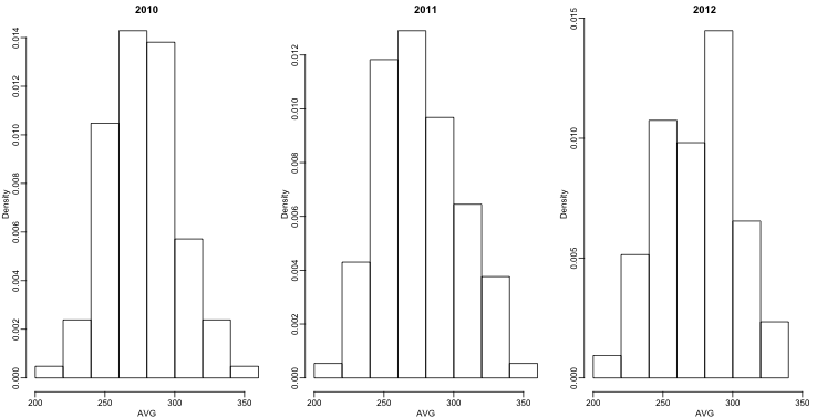
Batting average histograms for 2010, 2011, and 2012.

We note that the average player had an AVG of .275 and the standard deviation of the population of players was 0.027. So we can see already that .450 would be quite an anomaly since it is over six SDs away from the mean. So is José lucky or the best batter seen in the last 50 years? Perhaps it’s a combination of both. But how lucky and how good is he? If we become convinced that he is lucky, we should trade him to a team that trusts the .450 observation and is maybe overestimating his potential.

The hierarchical model

The hierarchical model provides a mathematical description of how we came to see the observation of .450. First, we pick a player at random with an intrinsic ability summarized by, for example, $\theta$ , then we see 20 random outcomes with success probability $\theta$ .

$\begin{align*} \theta &\sim N(\mu, \tau^2) \mbox{ describes randomness in picking a player}\\ Y \mid \theta &\sim N(\theta, \sigma^2) \mbox{ describes randomness in the performance of this particular player} \end{align*}$

Note the two levels (this is why we call them hierarchical): 1) Player to player variability and 2) variability due to luck when batting. In a Bayesian framework, the first level is called a prior distribution and the second the sampling distribution.

Now, let’s use this model for José’s data. Suppose we want to predict his innate ability in the form of his true batting average $\theta$ . This would be the hierarchical model for our data:

$\begin{align*} \theta &\sim N(.275, .027^2) \\ Y \mid \theta &\sim N(\theta, .110^2) \end{align*}$

We now are ready to compute a posterior distribution to summarize our prediction of $\theta$ . The continuous version of Bayes rule can be used here to derive the posterior probability, which is the distribution of the parameter $\theta$ given the observed data:

$\begin{align*} f_{ \theta \mid Y} (\theta\mid Y) &= \frac{f_{Y\mid \theta}(Y\mid \theta) f_{\theta}(\theta) }{f_Y(Y)}\\ &= \frac{f_{Y\mid \theta}(Y\mid \theta) f_{\theta}(\theta)} {\int_{\theta}f_{Y\mid \theta}(Y\mid \theta)f_{\theta}(\theta)} \end{align*}$

We are particularly interested in the $\theta$ that maximizes the posterior probability $f_{\theta\mid Y}(\theta\mid Y)$ . In our case, we can show that the posterior is normal and we can compute the mean $\mbox{E}(\theta\mid y)$ and variance $\mbox{var}(\theta\mid y)$ . Specifically, we can show the average of this distribution is the following:

$\begin{align*} \mbox{E}(\theta\mid y) &= B \mu + (1-B) Y\\ &= \mu + (1-B)(Y-\mu)\\ B &= \frac{\sigma^2}{\sigma^2+\tau^2} \end{align*}$ It is a weighted average of the population average $\mu$ and the observed data $Y$ . The weight depends on the SD of the the population $\tau$ and the SD of our observed data $\sigma$ . This weighted average is sometimes referred to as shrinking because it shrinks estimates towards a prior mean. In the case of José Iglesias, we have:

$\begin{align*} \mbox{E}(\theta \mid Y=.450) &= B \times .275 + (1 - B) \times .450 \\ &= .275 + (1 - B)(.450 - .260) \\ B &=\frac{.110^2}{.110^2 + .027^2} = 0.943\\ \mbox{E}(\theta \mid Y=450) &\approx .285 \end{align*}$

The variance can be shown to be:

$\mbox{var}(\theta\mid y) = \frac{1}{1/\sigma^2+1/\tau^2} = \frac{1}{1/.110^2 + 1/.027^2} = 0.026$

So we started with a frequentist 95% confidence interval that ignored data from other players and summarized just José’s data: .450 $\pm$ 0.220. Then we used an Bayesian approach that incorporated data from other players and other years to obtain a posterior probability. This is actually referred to as an empirical Bayes approach because we used data to construct the prior. From the posterior we can report what is called a 95% credible interval by reporting a region, centered at the mean, with a 95% chance of occurring. In our case, this turns out to be: .285 $\pm$ 0.052.

The Bayesian credible interval suggests that if another team is impressed by the .450 observation, we should consider trading José as we are predicting he will be just slightly above average. Interestingly, the Red Sox traded José to the Detroit Tigers in July. Here are the José Iglesias batting averages for the next five months.

Month	At Bat	Hits	AVG
April	20	9	.450
May	26	11	.423
June	86	34	.395
July	83	17	.205
August	85	25	.294
September	50	10	.200
Total w/o April	330	97	.293

Although both intervals included the final batting average, the Bayesian credible interval provided a much more precise prediction. In particular, it predicted that he would not be as good the remainder of the season.