Visualizing NGS data

We will use the following libraries to demonstrate visualization of NGS data.

#biocLite("pasillaBamSubset")
#biocLite("TxDb.Dmelanogaster.UCSC.dm3.ensGene")
library(pasillaBamSubset)
library(TxDb.Dmelanogaster.UCSC.dm3.ensGene)
fl1 <- untreated1_chr4()
fl2 <- untreated3_chr4()

We will try four ways to look at NGS coverage: using the standalone Java program IGV, using simple plot commands, and using the Gviz and ggbio packages in Bioconductor.

IGV

Copy these files from the R library directory to the current working directory. First set the working directory to the source file location. We need to use the Rsamtools library to index the BAM files for using IGV.

file.copy(from=fl1,to=basename(fl1))

## [1] FALSE

file.copy(from=fl2,to=basename(fl2))

## [1] FALSE

library(Rsamtools)

## Loading required package: Biostrings

## Loading required package: XVector

indexBam(basename(fl1))

##       untreated1_chr4.bam 
## "untreated1_chr4.bam.bai"

indexBam(basename(fl2))

##       untreated3_chr4.bam 
## "untreated3_chr4.bam.bai"

IGV is freely available for download here: https://www.broadinstitute.org/igv/home

You will need to provide an email, and then you will get a download link.

Using IGV, look for gene lgs.

Note that if you have trouble downloading IGV, another option for visualization is the UCSC Genome Browser: http://genome.ucsc.edu/cgi-bin/hgTracks

The UCSC Genome Browser is a great resource, having many tracks involving gene annotations, conservation over multiple species, and the ENCODE epigenetic tracks already available. However, the UCSC Genome Browser requires that you upload your genomic files to their server, or put your data on a publicly available server. This is not always possible if you are working with confidential data.

Simple plot

Next we will look at the same gene using the simple plot function in R.

library(GenomicRanges)

Note: if you are using Bioconductor version 14, paired with R 3.1, you should also load this library. You do not need to load this library, and it will not be available to you, if you are using Bioconductor version 13, paired with R 3.0.x.

library(GenomicAlignments)

## Loading required package: SummarizedExperiment

We read in the alignments from the file fl1. Then we use the coverage function to tally up the basepair coverage. We then extract the subset of coverage which overlaps our gene of interest, and convert this coverage from an RleList into a numeric vector. Remember from Week 2, that Rle objects are compressed, such that repeating numbers are stored as a number and a length.

x <- readGAlignments(fl1)
xcov <- coverage(x)
z <- GRanges("chr4",IRanges(456500,466000))
# Bioconductor 2.14
xcov[z]

## RleList of length 1
## $$chr4
## integer-Rle of length 9501 with 1775 runs
##   Lengths: 1252   10   52    4    7    2 ...   10    7   12  392   75 1041
##   Values :    0    2    3    4    5    6 ...    3    2    1    0    1    0

# Bioconductor 2.13
xcov$chr4[ranges(z)]

## integer-Rle of length 9501 with 1775 runs
##   Lengths: 1252   10   52    4    7    2 ...   10    7   12  392   75 1041
##   Values :    0    2    3    4    5    6 ...    3    2    1    0    1    0

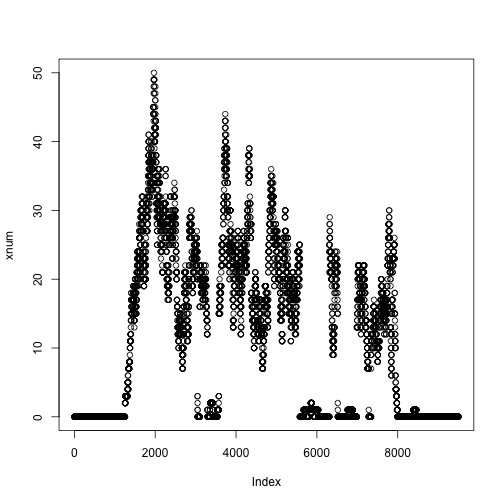
xnum <- as.numeric(xcov$chr4[ranges(z)])
plot(xnum)

plot of chunk unnamed-chunk-5

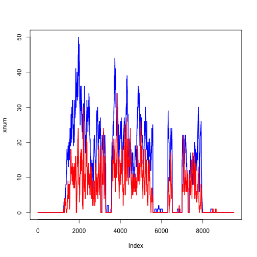
We can do the same for another file:

y <- readGAlignmentPairs(fl2)

## Warning in .make_GAlignmentPairs_from_GAlignments(gal, strandMode = strandMode, : 63 pairs (0 proper, 63 not proper) were dropped because the seqname
##   or strand of the alignments in the pair were not concordant.
##   Note that a GAlignmentPairs object can only hold concordant pairs at the
##   moment, that is, pairs where the 2 alignments are on the opposite strands
##   of the same reference sequence.

ycov <- coverage(y)
ynum <- as.numeric(ycov$chr4[ranges(z)])
plot(xnum, type="l", col="blue", lwd=2)
lines(ynum, col="red", lwd=2)

plot of chunk unnamed-chunk-6

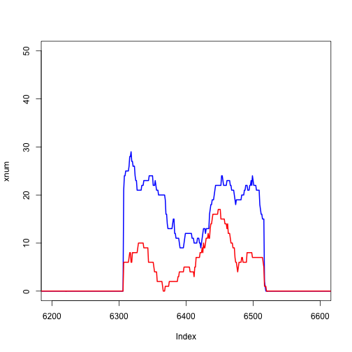
We can zoom in on a single exon:

plot(xnum, type="l", col="blue", lwd=2, xlim=c(6200,6600))
lines(ynum, col="red", lwd=2)

plot of chunk unnamed-chunk-7

Extracting the gene of interest using the transcript database

Suppose we are interested in visualizing the gene lgs. We can extract it from the transcript database TxDb.Dmelanogaster.UCSC.dm3.ensGene on Bioconductor, but first we need to look up the Ensembl gene name. We will use the functions that we learned in Week 7 to find the name.

# biocLite("biomaRt")
library(biomaRt)
m <- useMart("ensembl", dataset = "dmelanogaster_gene_ensembl")
lf <- listFilters(m)
lf[grep("name", lf$description, ignore.case=TRUE),]

##                             name
## 1                chromosome_name
## 17         with_flybasename_gene
## 19   with_flybasename_transcript
## 23  with_flybasename_translation
## 52            external_gene_name
## 66              flybasename_gene
## 67        flybasename_transcript
## 68       flybasename_translation
## 93                 wikigene_name
## 107               go_parent_name
## 208               so_parent_name
##                                      description
## 1                                Chromosome name
## 17                   with FlyBaseName gene ID(s)
## 19             with FlyBaseName transcript ID(s)
## 23                with FlyBaseName protein ID(s)
## 52          Associated Gene Name(s) [e.g. BRCA2]
## 66           FlyBaseName Gene ID(s) [e.g. cul-2]
## 67  FlyBaseName Transcript ID(s) [e.g. cul-2-RB]
## 68     FlyBaseName Protein ID(s) [e.g. cul-2-PB]
## 93                 WikiGene Name(s) [e.g. Ir21a]
## 107                             Parent term name
## 208                             Parent term name

map <- getBM(mart = m,
  attributes = c("ensembl_gene_id", "flybasename_gene"),
  filters = "flybasename_gene", 
  values = "lgs")
map

##   ensembl_gene_id flybasename_gene
## 1     FBgn0039907              lgs

Now we extract the exons for each gene, and then the exons for the gene lgs.

library(GenomicFeatures)
grl <- exonsBy(TxDb.Dmelanogaster.UCSC.dm3.ensGene, by="gene")
gene <- grl[[map$ensembl_gene_id[1]]]
gene

## GRanges object with 6 ranges and 2 metadata columns:
##       seqnames           ranges strand |   exon_id   exon_name
##          <Rle>        <IRanges>  <Rle> | <integer> <character>
##   [1]     chr4 [457583, 459544]      - |     63350        <NA>
##   [2]     chr4 [459601, 459791]      - |     63351        <NA>
##   [3]     chr4 [460074, 462077]      - |     63352        <NA>
##   [4]     chr4 [462806, 463015]      - |     63353        <NA>
##   [5]     chr4 [463490, 463780]      - |     63354        <NA>
##   [6]     chr4 [463839, 464533]      - |     63355        <NA>
##   -------
##   seqinfo: 15 sequences (1 circular) from dm3 genome

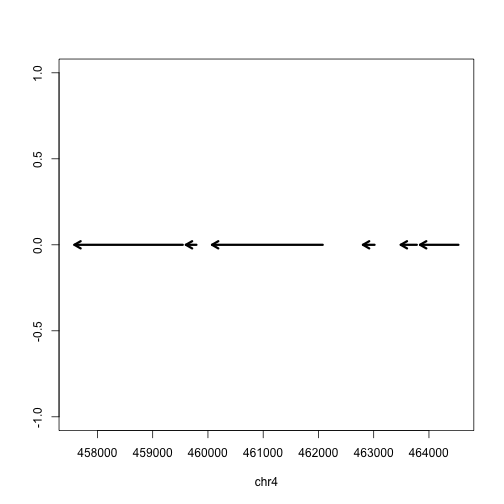
Finally we can plot these ranges to see what it looks like:

rg <- range(gene)
plot(c(start(rg), end(rg)), c(0,0), type="n", xlab=seqnames(gene)[1], ylab="")
arrows(start(gene),rep(0,length(gene)),
       end(gene),rep(0,length(gene)),
       lwd=3, length=.1)

plot of chunk unnamed-chunk-10

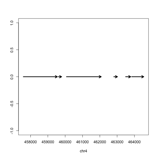
But actually, the gene is on the minus strand. We should add a line which corrects for minus strand genes:

plot(c(start(rg), end(rg)), c(0,0), type="n", xlab=seqnames(gene)[1], ylab="")
arrows(start(gene),rep(0,length(gene)),
       end(gene),rep(0,length(gene)),
       lwd=3, length=.1, 
       code=ifelse(as.character(strand(gene)[1]) == "+", 2, 1))

plot of chunk unnamed-chunk-11

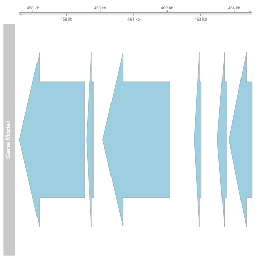
Gviz

We will briefly show two packages for visualizing genomic data in Bioconductor. Note that each of these have extensive vignettes for plotting many kinds of data. We will show here how to make the coverage plots as before:

#biocLite("Gviz")
library(Gviz)

## Loading required package: grid

gtrack <- GenomeAxisTrack()
atrack <- AnnotationTrack(gene, name = "Gene Model")
plotTracks(list(gtrack, atrack))

plot of chunk unnamed-chunk-12

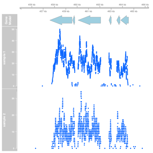
Extract the coverage. Gviz expects that data will be provided as GRanges objects, so we convert the RleList coverage to a GRanges object:

xgr <- as(xcov, "GRanges")
ygr <- as(ycov, "GRanges")
dtrack1 <- DataTrack(xgr[xgr %over% z], name = "sample 1")
dtrack2 <- DataTrack(ygr[ygr %over% z], name = "sample 2")
plotTracks(list(gtrack, atrack, dtrack1, dtrack2))

plot of chunk unnamed-chunk-13

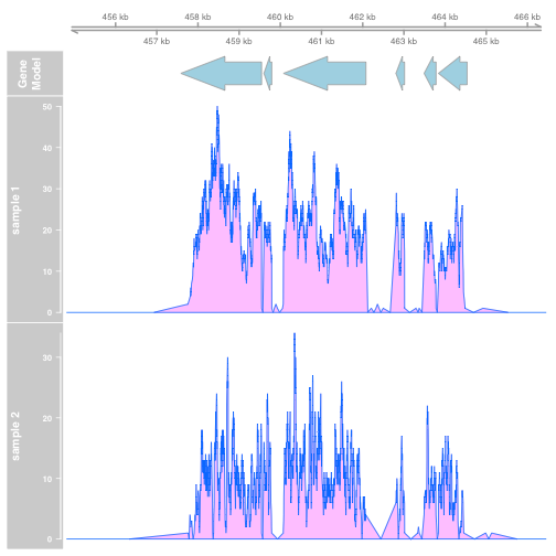
plotTracks(list(gtrack, atrack, dtrack1, dtrack2), type="polygon")

plot of chunk unnamed-chunk-13

ggbio

#biocLite("ggbio")
library(ggbio)

## Loading required package: ggplot2

## Warning: replacing previous import by 'BiocGenerics::Position' when loading
## 'ggbio'

## Need specific help about ggbio? try mailing 
##  the maintainer or visit http://tengfei.github.com/ggbio/

## 
## Attaching package: 'ggbio'

## The following objects are masked from 'package:ggplot2':
## 
##     geom_bar, geom_rect, geom_segment, ggsave, stat_bin,
##     stat_identity, xlim