Distance and Dimension Reduction

Introduction

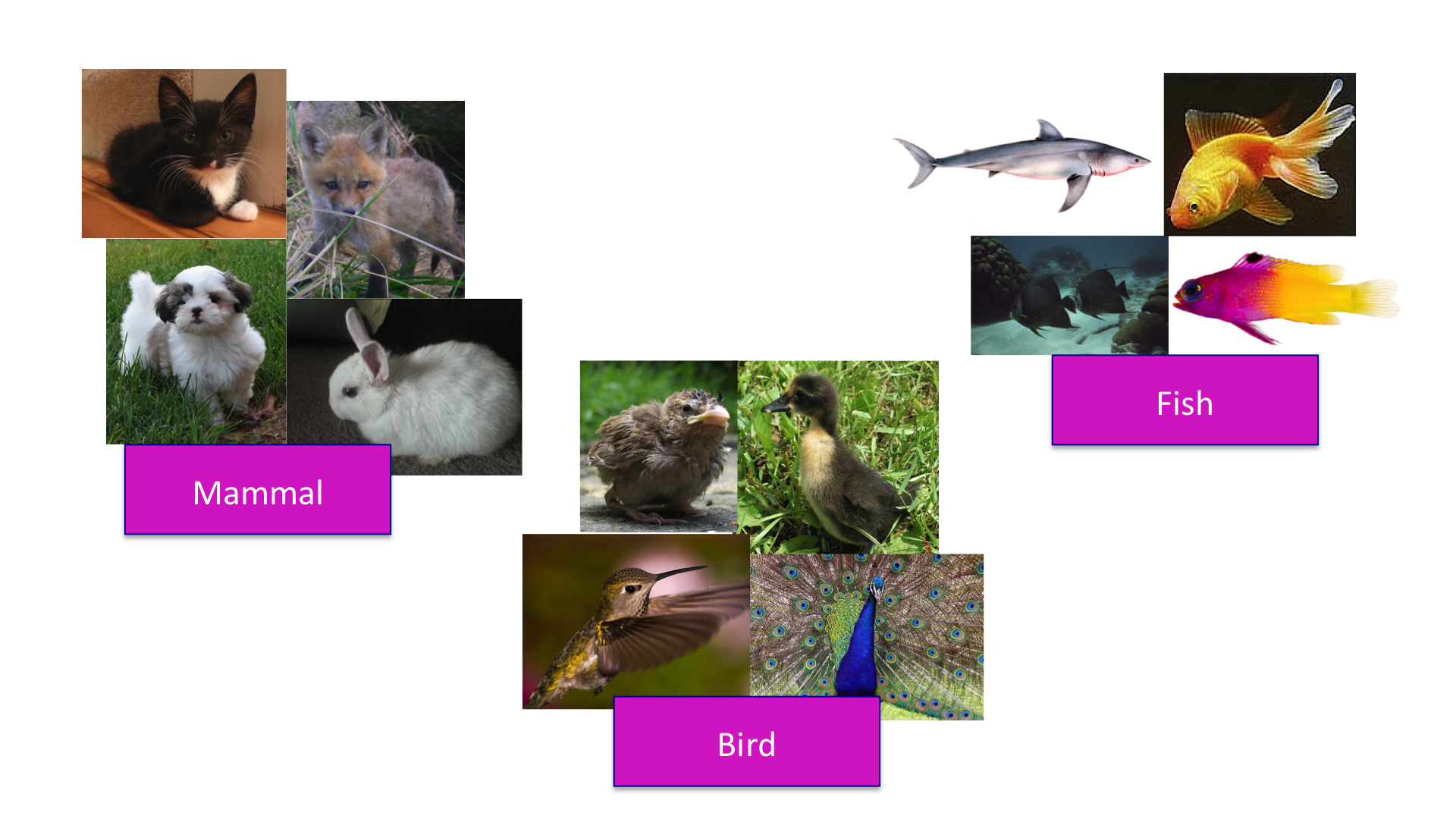
The concept of distance is quite intuitive. For example, when we cluster animals into subgroups, we are implicitly defining a distance that permits us to say what animals are “close” to each other.

Clustering of animals

Many of the analyses we perform with high-dimensional data relate directly or indirectly to distance. Many clustering and machine learning techniques rely on being able to define distance, using features or predictors. For example, to create heatmaps, which are widely used in genomics and other highthroughput fields, a distance is computed explicitly.

Example of heatmap

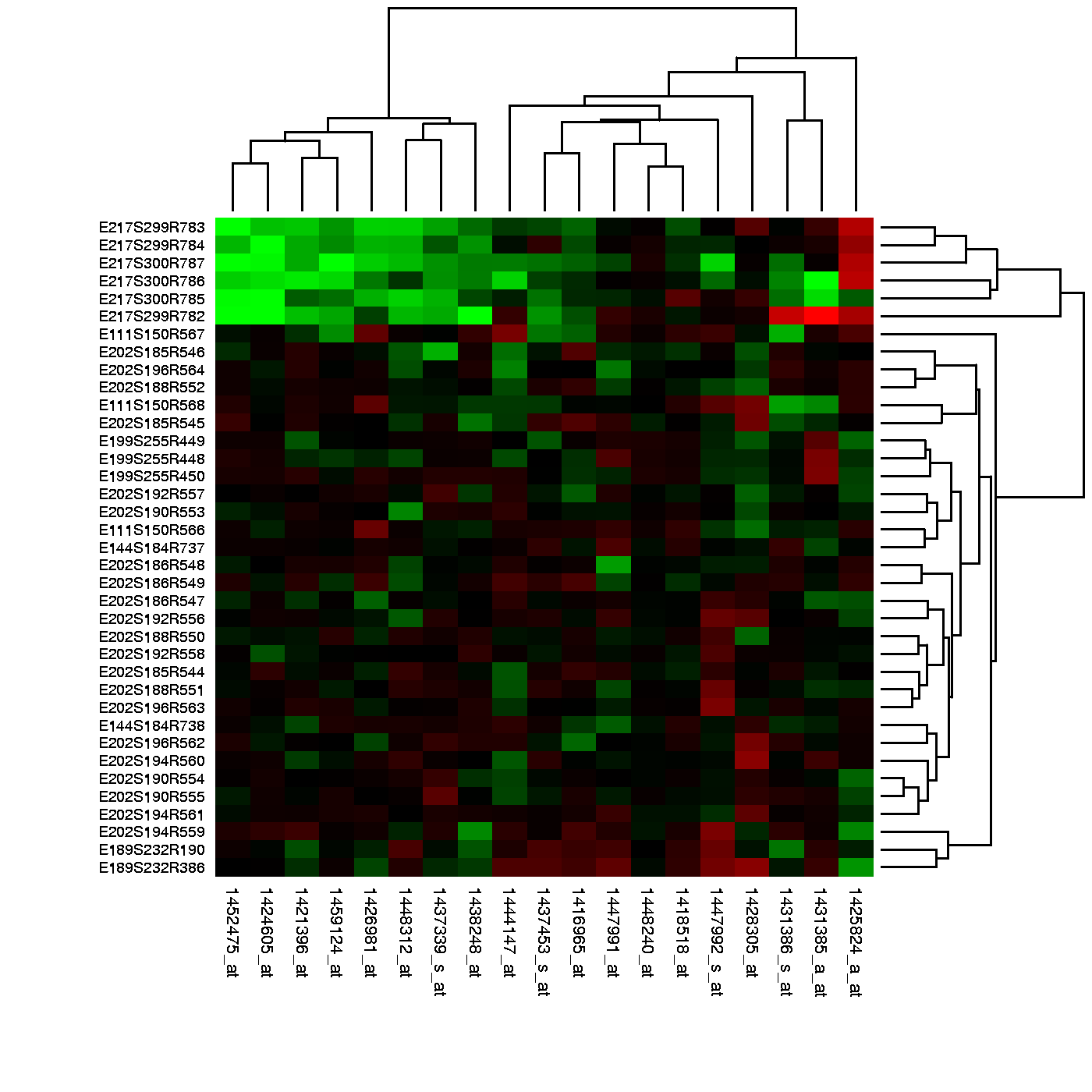
Image Source: Heatmap, Gaeddal, 01.28.2007

In these plots the measurements, which are stored in a matrix, are represented with colors after the columns and rows have been clustered. (A side note: red and green, a common color theme for heatmaps, are two of the most difficult colors for many color-blind people to discern.) Here we will learn the necessary mathematics and computing skills to understand and create heatmaps. We start by reviewing the mathematical definition of distance.

Euclidean Distance

As a review, let’s define the distance between two points, $A$ and $B$ , on a Cartesian plane.

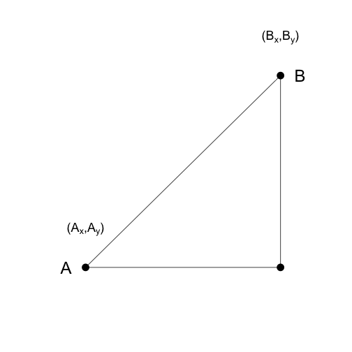
The euclidean distance between $A$ and $B$ is simply:

$\sqrt{ (A_x-B_x)^2 + (A_y-B_y)^2}$

Distance in High Dimensions

We introduce a dataset with gene expression measurements for 22,215 genes from 189 samples. The R objects can be downloaded like this:

library(devtools)
install_github("genomicsclass/tissuesGeneExpression")

The data represent RNA expression levels for eight tissues, each with several individuals.

library(tissuesGeneExpression)
data(tissuesGeneExpression)
dim(e) ##e contains the expression data

## [1] 22215   189

table(tissue) ##tissue[i] tells us what tissue is represented by e[,i]

## tissue
##  cerebellum       colon endometrium hippocampus      kidney       liver 
##          38          34          15          31          39          26 
##    placenta 
##           6

We are interested in describing distance between samples in the context of this dataset. We might also be interested in finding genes that behave similarly across samples.

To define distance, we need to know what the points are since mathematical distance is computed between points. With high dimensional data, points are no longer on the Cartesian plane. Instead they are in higher dimensions. For example, sample $i$ is defined by a point in 22,215 dimensional space: $(Y_{1,i},\dots,Y_{22215,i})^\top$ . Feature $g$ is defined by a point in 189 dimensions $(Y_{g,189},\dots,Y_{g,189})^\top$

Once we define points, the Euclidean distance is defined in a very similar way as it is defined for two dimensions. For instance, the distance between two samples $i$ and $j$ is:

$\mbox{dist}(i,j) = \sqrt{ \sum_{g=1}^{22215} (Y_{g,i}-Y_{g,j })^2 }$

and the distance between two features $h$ and $g$ is:

$\mbox{dist}(h,g) = \sqrt{ \sum_{i=1}^{189} (Y_{h,i}-Y_{g,i})^2 }$

Distance with matrix algebra

The distance between samples $i$ and $j$ can be written as

$\mbox{dist}(i,j) = (\mathbf{Y}_i - \mathbf{Y}_j)^\top(\mathbf{Y}_i - \mathbf{Y}_j)$

with $\mathbf{Y}_i$ and $\mathbf{Y}_j$ columns $i$ and $j$ . This result can be very convenient in practice as computations can be made much faster using matrix multiplication.

Examples

We can now use the formulas above to compute distance. Let’s compute distance between samples 1 and 2, both kidneys, and then to sample 87, a colon.

x <- e[,1]
y <- e[,2]
z <- e[,87]
sqrt(sum((x-y)^2))

## [1] 85.8546

sqrt(sum((x-z)^2))

## [1] 122.8919

As expected, the kidneys are closer to each other. A faster way to compute this is using matrix algebra:

sqrt( crossprod(x-y) )

##         [,1]
## [1,] 85.8546

sqrt( crossprod(x-z) )

##          [,1]
## [1,] 122.8919

Now to compute all the distances at once, we have the function dist. Because it computes the distance between each row, and here we are interested in the distance between samples, we transpose the matrix

d <- dist(t(e))
class(d)

## [1] "dist"

Note that this produces an object of class dist and, to access the entries using row and column, indexes we need to coerce it into a matrix:

as.matrix(d)[1,2]

## [1] 85.8546

as.matrix(d)[1,87]

## [1] 122.8919

It is important to remember that if we run dist on e, it will compute all pairwise distances between genes. This will try to create a $22215 \times 22215$ matrix that may crash your R sessions.

Distance lecture