Batch Effects

One often overlooked complication with high-throughput studies is batch effects, which occur because measurements are affected by laboratory conditions, reagent lots, and personnel differences. This becomes a major problem when batch effects are confounded with an outcome of interest and lead to incorrect conclusions. In this chapter, we describe batch effects in detail: how to detect, interpret, model, and adjust for batch effects.

Batch effects are the biggest challenge faced by genomics research, especially in the context of precision medicine. The presence of batch effects in one form or another have been reported among most, if not all, high-throughput technologies [Leek et al. (2010) Nature Reviews Genetics 11, 733-739]. But batch effects are not specific to genomics technology. In fact, in a 1972 paper, WJ Youden describes batch effects in the context of empirical estimates of physical constants. He pointed out the “subjective character of present estimates” of physical constants and how estimates changed from laboratory to laboratory. For example, in Table 1, Youden shows the following estimates of the astronomical unit from different laboratories. The reports included an estimate of spread (what we now would call a confidence interval).

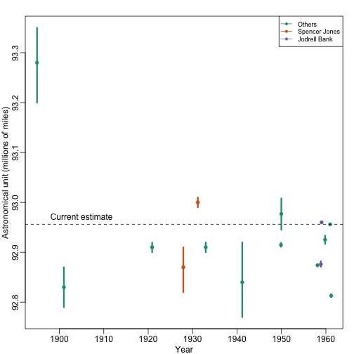
Estimates of the astronomical unit with estimates of spread, versus year it was reported. The two laboratories that reported more than one estimate are shown in color.

Judging by the variability across labs and the fact that the reported bounds do not explain this variability, clearly shows the presence of an effect that differs across labs, but not within. This type of variability is what we call a batch effect. Note that there are laboratories that reported two estimates (purple and orange) and batch effects are seen across the two different measurements from the same laboratories as well.

We can use statistical notation to precisely describe the problem. The scientists making these measurements assumed they observed:

$Y_{i,j} = \mu + \varepsilon_{i,j}, j=1,\dots,N$

with $Y_{i,j}$ the $j$ -th measurement of laboratory $i$ , $\mu$ the true physical constant, and $\varepsilon_{i,j}$ independent measurement error. To account for the variability introduced by $\varepsilon_{i,j}$ , we compute standard errors from the data. As we saw earlier in the book, we estimate the physical constant with the average of the $N$ measurements…

$\bar{Y}_i = \frac{1}{N} \sum_{i=1}^{N} Y_{i,j}$

.. and we can construct a confidence interval by:

$\bar{Y}_i \pm 2 s_i / \sqrt{N} \mbox{ with } s_i^2= \frac{1}{N-1} \sum_{i=1}^N (Y_{i,j} - \bar{Y}_i)^2$

However, this confidence interval will be too small because it does not catch the batch effect variability. A more appropriate model is:

$Y_{i,j} = \mu + \gamma_i + \varepsilon_{i,j}, j=1, \dots, N$

with $\gamma_i$ a laboratory specific bias or batch effect.

From the plot it is quite clear that the variability of $\gamma$ across laboratories is larger than the variability of $\varepsilon$ within a lab. The problem here is that there is no information about $\gamma$ in the data from a single lab. The statistical term for the problem is that $\mu$ and $\gamma$ are unidentifiable. We can estimate the sum $\mu_i+\gamma_i$ , but we can’t distinguish one from the other.

We can also view $\gamma$ as a random variable. In this case, each laboratory has an error term $\gamma_i$ that is the same across measurements from that lab, but different from lab to lab. Under this interpretation the problem is that:

$s_i / \sqrt{N} \mbox{ with } s_i^2= \frac{1}{N-1} \sum_{i=1}^N (Y_{ij} - \bar{Y}_i)^2$

is an underestimate of the standard error since it does not account for the within lab correlation induced by $\gamma$ .

With data from several laboratories we can in fact estimate the $\gamma$ , if we assume they average out to 0. Or we can consider them to be random effects and simply estimate a new estimate and standard error with all measurements. Here is a confidence interval treating each reported average as a random observation:

avg <- mean(dat[,3])
se <- sd(dat[,3]) / sqrt(nrow(dat))

## 95% confidence interaval is: [ 92.8727 , 92.98542 ]

## which does include the current estimate is: 92.95604

Youden’s paper also includes batch effect examples from more recent estimates of the speed of light, as well as estimates of the gravity constant. Here we demonstrate the widespread presence and complex nature of batch effects in high-throughput biological measurements.