The QR decomposition

The QR Factorization (Advanced)

We have seen that in order to calculate the LSE, we need to invert a matrix. In previous sections we used the function solve. However, solve is not a stable solution. When coding LSE computation, we use the QR decomposition.

Inverting $\mathbf{X^\top X}$

Remember that to minimize the RSS:

$(\mathbf{Y}-\mathbf{X}\boldsymbol{\beta})^\top (\mathbf{Y}-\mathbf{X}\boldsymbol{\beta})$

We need to solve:

$\mathbf{X}^\top \mathbf{X} \boldsymbol{\hat{\beta}} = \mathbf{X}^\top \mathbf{Y}$

The solution is:

$\boldsymbol{\hat{\beta}} = (\mathbf{X}^\top \mathbf{X})^{-1} \mathbf{X}^\top \mathbf{Y}$

Thus, we need to compute $(\mathbf{X}^\top \mathbf{X})^{-1}$ .

`solve` is numerically unstable

To demonstrate what we mean by numerically unstable, we construct an extreme case:

n <- 50;M <- 500
x <- seq(1,M,len=n)
X <- cbind(1,x,x^2,x^3)
colnames(X) <- c("Intercept","x","x2","x3")
beta <- matrix(c(1,1,1,1),4,1)
set.seed(1)
y <- X%*%beta+rnorm(n,sd=1)

The standard R function for inverse gives an error:

solve(crossprod(X)) %*% crossprod(X,y)

To see why this happens, look at $(\mathbf{X}^\top \mathbf{X})$

options(digits=4)
log10(crossprod(X))

##           Intercept      x     x2     x3
## Intercept     1.699  4.098  6.625  9.203
## x             4.098  6.625  9.203 11.810
## x2            6.625  9.203 11.810 14.434
## x3            9.203 11.810 14.434 17.070

Note the difference of several orders of magnitude. On a digital computer, we have a limited range of numbers. This makes some numbers seem like 0, when we also have to consider very large numbers. This in turn leads to divisions that are practically divisions by 0 errors.

The factorization

The QR factorization is based on a mathematical result that tells us that we can decompose any full rank $N\times p$ matrix $\mathbf{X}$ as:

$\mathbf{X = QR}$

with:

$\mathbf{Q}$ a $N \times p$ matrix with $\mathbf{Q^\top Q=I}$
$\mathbf{R}$ a $p \times p$ upper triangular matrix.

Upper triangular matrices are very convenient for solving system of equations.

Example of upper triangular matrix

In the example below, the matrix on the left is upper triangular: it only has 0s below the diagonal. This facilitates solving the system of equations greatly:

$\, \begin{pmatrix} 1&2&-1\\ 0&1&2\\ 0&0&1\\ \end{pmatrix} \begin{pmatrix} a\\ b\\ c\\ \end{pmatrix} = \begin{pmatrix} 6\\ 4\\ 1\\ \end{pmatrix}$

We immediately know that $c=1$ , which implies that $b+2=4$ . This in turn implies $b=2$ and thus $a+4-1=6$ so $a = 3$ . Writing an algorithm to do this is straight-forward for any upper triangular matrix.

Finding LSE with QR

If we rewrite the equations of the LSE using $\mathbf{QR}$ instead of $\mathbf{X}$ we have:

$\mathbf{X}^\top \mathbf{X} \boldsymbol{\beta} = \mathbf{X}^\top \mathbf{Y}$ $(\mathbf{Q}\mathbf{R})^\top (\mathbf{Q}\mathbf{R}) \boldsymbol{\beta} = (\mathbf{Q}\mathbf{R})^\top \mathbf{Y}$ $\mathbf{R}^\top (\mathbf{Q}^\top \mathbf{Q}) \mathbf{R} \boldsymbol{\beta} = \mathbf{R}^\top \mathbf{Q}^\top \mathbf{Y}$ $\mathbf{R}^\top \mathbf{R} \boldsymbol{\beta} = \mathbf{R}^\top \mathbf{Q}^\top \mathbf{Y}$ $(\mathbf{R}^\top)^{-1} \mathbf{R}^\top \mathbf{R} \boldsymbol{\beta} = (\mathbf{R}^\top)^{-1} \mathbf{R}^\top \mathbf{Q}^\top \mathbf{Y}$ $\mathbf{R} \boldsymbol{\beta} = \mathbf{Q}^\top \mathbf{Y}$

$\mathbf{R}$ being upper triangular makes solving this more stable. Also, because $\mathbf{Q}^\top\mathbf{Q}=\mathbf{I}$ , we know that the columns of $\mathbf{Q}$ are in the same scale which stabilizes the right side.

Now we are ready to find LSE using the QR decomposition. To solve:

$\mathbf{R} \boldsymbol{\beta} = \mathbf{Q}^\top \mathbf{Y}$

We use backsolve which takes advantage of the upper triangular nature of $\mathbf{R}$ .

QR <- qr(X)
Q <- qr.Q( QR )
R <- qr.R( QR )
(betahat <- backsolve(R, crossprod(Q,y) ) )

##        [,1]
## [1,] 0.9038
## [2,] 1.0066
## [3,] 1.0000
## [4,] 1.0000

In practice, we do not need to do any of this due to the built-in solve.qr function:

QR <- qr(X)
(betahat <- solve.qr(QR, y))

##             [,1]
## Intercept 0.9038
## x         1.0066
## x2        1.0000
## x3        1.0000

Fitted values

This factorization also simplifies the calculation for fitted values:

$\mathbf{X}\boldsymbol{\hat{\beta}} = (\mathbf{QR})\mathbf{R}^{-1}\mathbf{Q}^\top \mathbf{y}= \mathbf{Q}\mathbf{Q}^\top\mathbf{y}$

In R, we simply do the following:

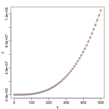
library(rafalib)
mypar(1,1)
plot(x,y)
fitted <- tcrossprod(Q)%*%y
lines(x,fitted,col=2)

plot of chunk unnamed-chunk-7

Standard errors

To obtain the standard errors of the LSE, we note that:

$(\mathbf{X^\top X})^{-1} = (\mathbf{R^\top Q^\top QR})^{-1} = (\mathbf{R^\top R})^{-1}$

The function chol2inv is specifically designed to find this inverse. So all we do is the following:

df <- length(y) - QR$rank
sigma2 <- sum((y-fitted)^2)/df
varbeta <- sigma2*chol2inv(qr.R(QR))
SE <- sqrt(diag(varbeta))
cbind(betahat,SE)

##                         SE
## Intercept 0.9038 4.508e-01
## x         1.0066 7.858e-03
## x2        1.0000 3.662e-05
## x3        1.0000 4.802e-08

This gives us identical results to the lm function.

summary(lm(y~0+X))$coef

##            Estimate Std. Error   t value   Pr(>|t|)
## XIntercept   0.9038  4.508e-01 2.005e+00  5.089e-02
## Xx           1.0066  7.858e-03 1.281e+02  2.171e-60
## Xx2          1.0000  3.662e-05 2.731e+04 1.745e-167
## Xx3          1.0000  4.802e-08 2.082e+07 4.559e-300