NGS read counting
The following lab will describe how to count NGS reads which fall into genomic features. We want to end up with a count matrix which has rows corresponding to genomic ranges and columns which correspond to different experiments or samples. As an example, we will use an RNA-Seq experiment, with files in the pasillaBamSubset Bioconductor data package. However, the same functions can be used for DNA-Seq, ChIP-Seq, etc.
#biocLite("pasillaBamSubset")
#biocLite("TxDb.Dmelanogaster.UCSC.dm3.ensGene")
library(pasillaBamSubset)
library(TxDb.Dmelanogaster.UCSC.dm3.ensGene)
We load a transcript database object. These are prebuilt in R for various well studied organisms, for example TxDb.Hsapiens.UCSC.hg19.knownGene. In addition the makeTranscriptDbFromGFF file can be used to import GFF or GTF gene models. We use the exonsBy function to get a GRangesList object of the exons for each gene.
txdb <- TxDb.Dmelanogaster.UCSC.dm3.ensGene
grl <- exonsBy(txdb, by="gene")
grl[100]
## GRangesList object of length 1:
## $$FBgn0000286
## GRanges object with 8 ranges and 2 metadata columns:
##       seqnames             ranges strand |   exon_id   exon_name
##          <Rle>          <IRanges>  <Rle> | <integer> <character>
##   [1]    chr2L [4876890, 4879196]      - |      8515        <NA>
##   [2]    chr2L [4877289, 4879196]      - |      8516        <NA>
##   [3]    chr2L [4880294, 4880472]      - |      8517        <NA>
##   [4]    chr2L [4880378, 4880472]      - |      8518        <NA>
##   [5]    chr2L [4881215, 4882492]      - |      8519        <NA>
##   [6]    chr2L [4882865, 4883113]      - |      8520        <NA>
##   [7]    chr2L [4882889, 4883113]      - |      8521        <NA>
##   [8]    chr2L [4882889, 4883341]      - |      8522        <NA>
##
## -------
## seqinfo: 15 sequences (1 circular) from dm3 genome
grl[[100]]
## GRanges object with 8 ranges and 2 metadata columns:
##       seqnames             ranges strand |   exon_id   exon_name
##          <Rle>          <IRanges>  <Rle> | <integer> <character>
##   [1]    chr2L [4876890, 4879196]      - |      8515        <NA>
##   [2]    chr2L [4877289, 4879196]      - |      8516        <NA>
##   [3]    chr2L [4880294, 4880472]      - |      8517        <NA>
##   [4]    chr2L [4880378, 4880472]      - |      8518        <NA>
##   [5]    chr2L [4881215, 4882492]      - |      8519        <NA>
##   [6]    chr2L [4882865, 4883113]      - |      8520        <NA>
##   [7]    chr2L [4882889, 4883113]      - |      8521        <NA>
##   [8]    chr2L [4882889, 4883341]      - |      8522        <NA>
##   -------
##   seqinfo: 15 sequences (1 circular) from dm3 genome
grl[[100]][1]
## GRanges object with 1 range and 2 metadata columns:
##       seqnames             ranges strand |   exon_id   exon_name
##          <Rle>          <IRanges>  <Rle> | <integer> <character>
##   [1]    chr2L [4876890, 4879196]      - |      8515        <NA>
##   -------
##   seqinfo: 15 sequences (1 circular) from dm3 genome
These functions in the pasillaBamSubset package just point us to the BAM files.
fl1 <- untreated1_chr4()
fl2 <- untreated3_chr4()
fl1
## [1] "/usr/local/lib/R/site-library/pasillaBamSubset/extdata/untreated1_chr4.bam"
We need the following libraries for counting BAM files.
library(Rsamtools)
## Loading required package: XVector
## Loading required package: Biostrings
library(GenomicRanges)
library(GenomicAlignments)
We specify the files using the BamFileList function. For more fine grain control, you can tell the read counting functions how many reads to load at once with the yieldSize argument.
fls <- BamFileList(c(fl1, fl2))
names(fls) <- c("first","second")
The following function counts the overlaps of the reads in the BAM files in the features, which are the genes of Drosophila. We tell the counting function to ignore the strand, i.e., to allow minus strand reads to count in plus strand genes, and vice versa.
so1 <- summarizeOverlaps(features=grl,
                         reads=fls,
                         ignore.strand=TRUE)
so1
## class: SummarizedExperiment
## dim: 15682 2
## exptData(0):
## assays(1): counts
## rownames(15682): FBgn0000003 FBgn0000008 ... FBgn0264726
##   FBgn0264727
## rowData metadata column names(0):
## colnames(2): first second
## colData names(0):
We can examine the count matrix, which is stored in the assay slot:
head(assay(so1))
##             first second
## FBgn0000003     0      0
## FBgn0000008     0      0
## FBgn0000014     0      0
## FBgn0000015     0      0
## FBgn0000017     0      0
## FBgn0000018     0      0
colSums(assay(so1))
##  first second
## 156469 122872
The other parts of a SummarizedExperiment.
rowData(so1) # rowData will become rowRanges in the next release of Bioc
## GRangesList object of length 15682:
## $$FBgn0000003
## GRanges object with 1 range and 2 metadata columns:
##       seqnames             ranges strand |   exon_id   exon_name
##          <Rle>          <IRanges>  <Rle> | <integer> <character>
##   [1]    chr3R [2648220, 2648518]      + |     45123        <NA>
##
## $$FBgn0000008
## GRanges object with 13 ranges and 2 metadata columns:
##        seqnames               ranges strand   | exon_id exon_name
##    [1]    chr2R [18024494, 18024531]      +   |   20314      <NA>
##    [2]    chr2R [18024496, 18024713]      +   |   20315      <NA>
##    [3]    chr2R [18024938, 18025756]      +   |   20316      <NA>
##    [4]    chr2R [18025505, 18025756]      +   |   20317      <NA>
##    [5]    chr2R [18039159, 18039200]      +   |   20322      <NA>
##    ...      ...                  ...    ... ...     ...       ...
##    [9]    chr2R [18058283, 18059490]      +   |   20326      <NA>
##   [10]    chr2R [18059587, 18059757]      +   |   20327      <NA>
##   [11]    chr2R [18059821, 18059938]      +   |   20328      <NA>
##   [12]    chr2R [18060002, 18060339]      +   |   20329      <NA>
##   [13]    chr2R [18060002, 18060346]      +   |   20330      <NA>
##
## ...
## <15680 more elements>
## -------
## seqinfo: 15 sequences (1 circular) from dm3 genome
colData(so1)
## DataFrame with 2 rows and 0 columns
colData(so1)$sample <- c("one","two")
colData(so1)
## DataFrame with 2 rows and 1 column
##             sample
##        <character>
## first          one
## second         two
metadata(rowData(so1))
## $$genomeInfo
## $$genomeInfo$`Db type`
## [1] "TxDb"
##
## $$genomeInfo$`Supporting package`
## [1] "GenomicFeatures"
##
## $$genomeInfo$`Data source`
## [1] "UCSC"
##
## $$genomeInfo$Genome
## [1] "dm3"
##
## $$genomeInfo$Organism
## [1] "Drosophila melanogaster"
##
## $$genomeInfo$`UCSC Table`
## [1] "ensGene"
##
## $$genomeInfo$`Resource URL`
## [1] "http://genome.ucsc.edu/"
##
## $$genomeInfo$`Type of Gene ID`
## [1] "Ensembl gene ID"
##
## $$genomeInfo$`Full dataset`
## [1] "yes"
##
## $$genomeInfo$`miRBase build ID`
## [1] NA
##
## $$genomeInfo$transcript_nrow
## [1] "29173"
##
## $$genomeInfo$exon_nrow
## [1] "76920"
##
## $$genomeInfo$cds_nrow
## [1] "62135"
##
## $$genomeInfo$`Db created by`
## [1] "GenomicFeatures package from Bioconductor"
##
## $$genomeInfo$`Creation time`
## [1] "2014-09-26 11:22:16 -0700 (Fri, 26 Sep 2014)"
##
## $$genomeInfo$`GenomicFeatures version at creation time`
## [1] "1.17.17"
##
## $$genomeInfo$`RSQLite version at creation time`
## [1] "0.11.4"
##
## $$genomeInfo$DBSCHEMAVERSION
## [1] "1.0"
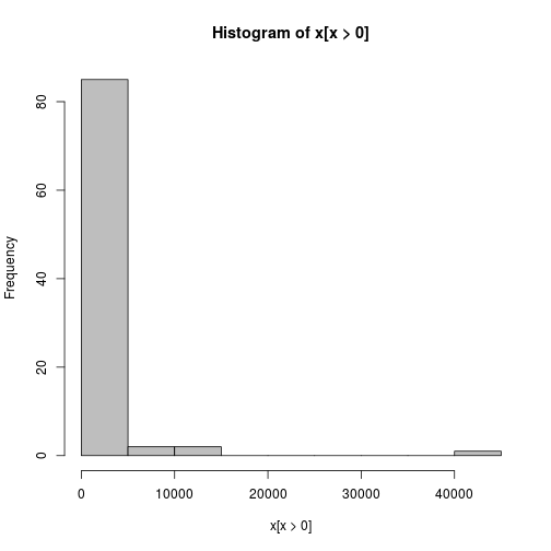
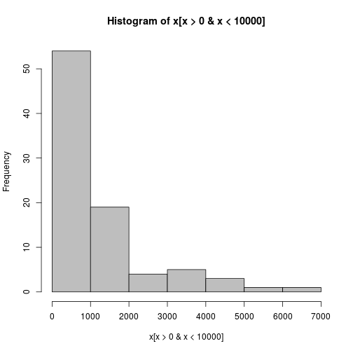
We can do some basic exploratory data analysis of the counts:
x <- assay(so1)[,1]
hist(x[x > 0], col="grey")
hist(x[x > 0 & x < 10000], col="grey")
plot(assay(so1) + 1, log="xy")

The second file should actually be counted in a special manner, as it contains pairs of reads which come from a single fragment. We do not want to count these twice, so we set singleEnd = FALSE. Additionally, we specify fragments = TRUE which counts reads if only one of the pair aligns to the features, and the other pair aligns to no feature.
# ?untreated3_chr4
# ?summarizeOverlaps
fls <- BamFileList(fl2)
so2 <- summarizeOverlaps(features=grl,
                         reads=fls,
                         ignore.strand=TRUE,
                         singleEnd=FALSE,
                         fragments=TRUE)
colSums(assay(so2))
## untreated3_chr4.bam
##               65591
colSums(assay(so1))
##  first second
## 156469 122872
plot(assay(so1)[,2], assay(so2)[,1], xlim=c(0,5000), ylim=c(0,5000),
     xlab="single end counting", ylab="paired end counting")
abline(0,1)
abline(0,.5)

Footnotes
Methods for counting reads which overlap features
Bioconductor packages:
summarizeOverlapsin theGenomicAlignmentspackage
http://www.bioconductor.org/packages/release/bioc/html/GenomicAlignments.html
featureCountsin theRsubreadpackage
Liao Y, Smyth GK, Shi W., “featureCounts: an efficient general purpose program for assigning sequence reads to genomic features.” Bioinformatics. 2014 http://www.ncbi.nlm.nih.gov/pubmed/24227677 http://bioinf.wehi.edu.au/featureCounts/
Command line tools:
htseq-count, a program in thehtseqPython package
Simon Anders, Paul Theodor Pyl, Wolfgang Huber. HTSeq — A Python framework to work with high-throughput sequencing data bioRxiv preprint (2014), doi: 10.1101/002824
http://www-huber.embl.de/users/anders/HTSeq/doc/count.html
-
bedtoolshttps://code.google.com/p/bedtools/