Smoothing

Smoothing is a very powerful technique used all across data analysis. It is designed to estimate $f(x)$ when the shape is unknown, but assumed to be smooth. The general idea is to group data points that are expected to have similar expectations and compute the average, or fit a simple parametric model. We illustrate two smoothing techniques using a gene expression example.

The following data are gene expression measurements from replicated RNA samples.

##Following three packages are available from Bioconductor
library(Biobase)
library(SpikeIn)
library(hgu95acdf)
data(SpikeIn95)

We consider the data used in an MA-plot comparing two replicated samples ( $Y$ = log ratios and $X$ = averages) and take down-sample in a way that balances the number of points for different strata of $X$ (code not shown):

library(rafalib)
mypar()
plot(X,Y)

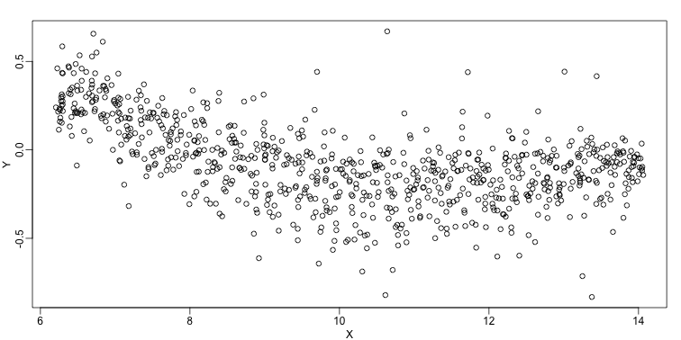
MAplot comparing gene expression from two arrays.

In the MA plot we see that $Y$ depends on $X$ . This dependence must be a bias because these are based on replicates, which means $Y$ should be 0 on average regardless of $X$ . We want to predict $f(x)=\mbox{E}(Y \mid X=x)$ so that we can remove this bias. Linear regression does not capture the apparent curvature in $f(x)$ :

mypar()
plot(X,Y)
fit <- lm(Y~X)
points(X,Y,pch=21,bg=ifelse(Y>fit$fitted,1,3))
abline(fit,col=2,lwd=4,lty=2)

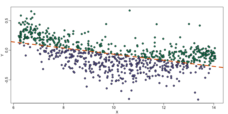
MAplot comparing gene expression from two arrays with fitted regression line. The two colors represent positive and negative residuals.

The points above the fitted line (green) and those below (purple) are not evenly distributed. We therefore need an alternative more flexible approach.

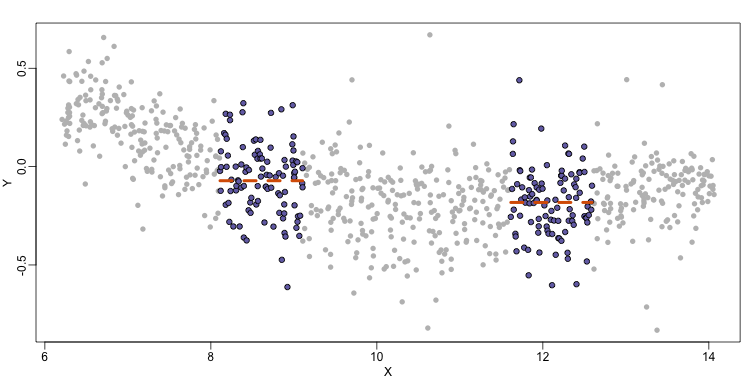
Bin Smoothing

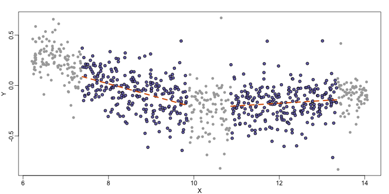
Instead of fitting a line, let’s go back to the idea of stratifying and computing the mean. This is referred to as bin smoothing. The general idea is that the underlying curve is “smooth” enough so that, in small bins, the curve is approximately constant. If we assume the curve is constant, then all the $Y$ in that bin have the same expected value. For example, in the plot below, we highlight points in a bin centered at 8.6, as well as the points of a bin centered at 12.1, if we use bins of size 1. We also show the fitted mean values for the $Y$ in those bins with dashed lines (code not shown):

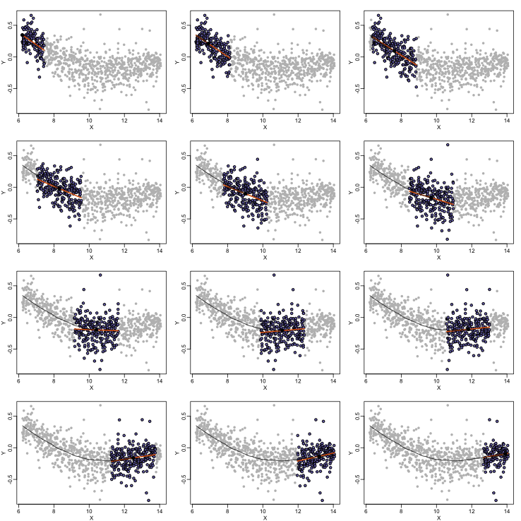
MAplot comparing gene expression from two arrays with bin smoother fit shown for two points.

By computing this mean for bins around every point, we form an estimate of the underlying curve $f(x)$ . Below we show the procedure happening as we move from the smallest value of $x$ to the largest. We show 10 intermediate cases as well (code not shown):

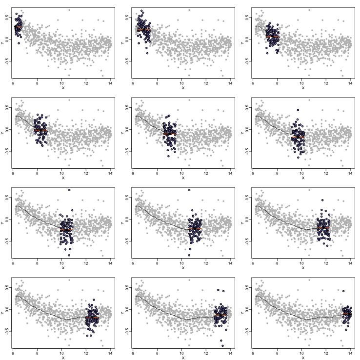
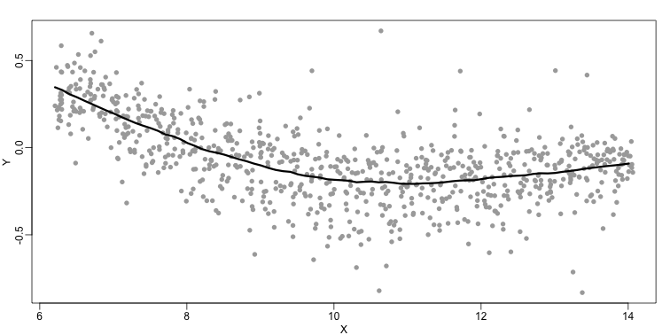
Illustration of how bin smoothing estimates a curve. howing in 12 steps of process.

The final result looks like this (code not shown):

MA-plot with curve obtained with bin smooth shown.

There are several functions in R that implement bin smoothers. One example is ksmooth. However, in practice, we typically prefer methods that use slightly more complicated models than fitting a constant. The final result above, for example, is somewhat wiggly. Methods such as loess, which we explain next, improve on this.

Loess

Local weighted regression (loess) is similar to bin smoothing in principle. The main difference is that we approximate the local behavior with a line or a parabola. This permits us to expand the bin sizes, which stabilizes the estimates. Below we see lines fitted to two bins that are slightly larger than those we used for the bin smoother (code not shown). We can use larger bins because fitting lines provide slightly more flexibility.

MAplot comparing gene expression from two arrays with bin local regression fit shown for two points.

As we did for the bin smoother, we show 12 steps of the process that leads to a loess fit (code not shown):

Illustration of how loess estimates a curves. Showing 12 steps of the process.

The final result is a smoother fit than the bin smoother since we use larger sample sizes to estimate our local parameters (code not shown):

MA-plot with curve obtained with by loess shown.

The function loess performs this analysis for us:

fit <- loess(Y~X, degree=1, span=1/3)

newx <- seq(min(X),max(X),len=100) 
smooth <- predict(fit,newdata=data.frame(X=newx))

mypar ()
plot(X,Y,col="darkgrey",pch=16)
lines(newx,smooth,col="black",lwd=3)

Loess fitted with the loess function.

There are three other important differences between loess and the typical bin smoother. The first is that rather than keeping the bin size the same, loess keeps the number of points used in the local fit the same. This number is controlled via the span argument which expects a proportion. For example, if N is the number of data points and span=0.5, then for a given $x$ , loess will use the 0.5*N closest points to $x$ for the fit. The second difference is that, when fitting the parametric model to obtain $f(x)$ , loess uses weighted least squares, with higher weights for points that are closer to $x$ . The third difference is that loess has the option of fitting the local model robustly. An iterative algorithm is implemented in which, after fitting a model in one iteration, outliers are detected and downweighted for the next iteration. To use this option, we use the argument family="symmetric".