Standard Errors

We have shown how to find the least squares estimates with matrix algebra. These estimates are random variables since they are linear combinations of the data. For these estimates to be useful, we also need to compute their standard errors. Linear algebra provides a powerful approach for this task. We provide several examples.

Falling object

It is useful to think about where randomness comes from. In our falling object example, randomness was introduced through measurement errors. Each time we rerun the experiment, a new set of measurement errors will be made. This implies that our data will change randomly, which in turn suggests that our estimates will change randomly. For instance, our estimate of the gravitational constant will change every time we perform the experiment. The constant is fixed, but our estimates are not. To see this we can run a Monte Carlo simulation. Specifically, we will generate the data repeatedly and each time compute the estimate for the quadratic term.

set.seed(1)
B <- 10000
h0 <- 56.67
v0 <- 0
g <- 9.8 ##meters per second

n <- 25
tt <- seq(0,3.4,len=n) ##time in secs, t is a base function
X <-cbind(1,tt,tt^2)
##create X'X^-1 X'
A <- solve(crossprod(X)) %*% t(X)
betahat<-replicate(B,{
  y <- h0 + v0*tt  - 0.5*g*tt^2 + rnorm(n,sd=1)
  betahats <- A%*%y
  return(betahats[3])
})
head(betahat)

## [1] -5.038646 -4.894362 -5.143756 -5.220960 -5.063322 -4.777521

As expected, the estimate is different every time. This is because $\hat{\beta}$ is a random variable. It therefore has a distribution:

library(rafalib)
mypar(1,2)
hist(betahat)
qqnorm(betahat)
qqline(betahat)

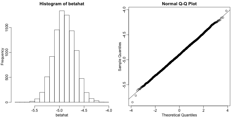
Distribution of estimated regression coefficients obtained from Monte Carlo simulated falling object data. The left is a histogram and on the right we have a qq-plot against normal theoretical quantiles.

Since $\hat{\beta}$ is a linear combination of the data which we made normal in our simulation, it is also normal as seen in the qq-plot above. Also, the mean of the distribution is the true parameter $-0.5g$ , as confirmed by the Monte Carlo simulation performed above.

round(mean(betahat),1)

## [1] -4.9

But we will not observe this exact value when we estimate because the standard error of our estimate is approximately:

sd(betahat) 

## [1] 0.2129976

Here we will show how we can compute the standard error without a Monte Carlo simulation. Since in practice we do not know exactly how the errors are generated, we can’t use the Monte Carlo approach.

Father and son heights

In the father and son height examples, we have randomness because we have a random sample of father and son pairs. For the sake of illustration, let’s assume that this is the entire population:

library(UsingR)
x <- father.son$fheight
y <- father.son$sheight
n <- length(y)

Now let’s run a Monte Carlo simulation in which we take a sample size of 50 over and over again.

N <- 50
B <-1000
betahat <- replicate(B,{
  index <- sample(n,N)
  sampledat <- father.son[index,]
  x <- sampledat$fheight
  y <- sampledat$sheight
  lm(y~x)$coef
  })
betahat <- t(betahat) #have estimates in two columns

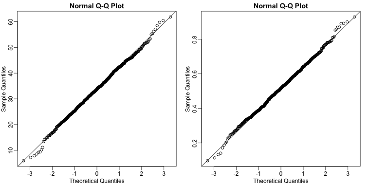
By making qq-plots, we see that our estimates are approximately normal random variables:

mypar(1,2)
qqnorm(betahat[,1])
qqline(betahat[,1])
qqnorm(betahat[,2])
qqline(betahat[,2])

Distribution of estimated regression coefficients obtained from Monte Carlo simulated father-son height data. The left is a histogram and on the right we have a qq-plot against normal theoretical quantiles.

We also see that the correlation of our estimates is negative:

cor(betahat[,1],betahat[,2])

## [1] -0.9992293

When we compute linear combinations of our estimates, we will need to know this information to correctly calculate the standard error of these linear combinations.

In the next section, we will describe the variance-covariance matrix. The covariance of two random variables is defined as follows:

mean( (betahat[,1]-mean(betahat[,1] ))* (betahat[,2]-mean(betahat[,2])))

## [1] -1.035291

The covariance is the correlation multiplied by the standard deviations of each random variable:

$\mbox{Corr}(X,Y) = \frac{\mbox{Cov}(X,Y)}{\sigma_X \sigma_Y}$

Other than that, this quantity does not have a useful interpretation in practice. However, as we will see, it is a very useful quantity for mathematical derivations. In the next sections, we show useful matrix algebra calculations that can be used to estimate standard errors of linear model estimates.

Variance-covariance matrix

As a first step we need to define the variance-covariance matrix, $\boldsymbol{\Sigma}$ . For a vector of random variables, $\mathbf{Y}$ , we define $\boldsymbol{\Sigma}$ as the matrix with the $i,j$ entry:

$\Sigma_{i,j} \equiv \mbox{Cov}(Y_i, Y_j)$

The covariance is equal to the variance if $i = j$ and equal to 0 if the variables are independent. In the kinds of vectors considered up to now, for example, a vector $\mathbf{Y}$ of individual observations $Y_i$ sampled from a population, we have assumed independence of each observation and assumed the $Y_i$ all have the same variance $\sigma^2$ , so the variance-covariance matrix has had only two kinds of elements:

$\mbox{Cov}(Y_i, Y_i) = \mbox{var}(Y_i) = \sigma^2$ $\mbox{Cov}(Y_i, Y_j) = 0, \mbox{ for } i \neq j$

which implies that $\boldsymbol{\Sigma} = \sigma^2 \mathbf{I}$ with $\mathbf{I}$ , the identity matrix.

Later, we will see a case, specifically the estimate coefficients of a linear model, $\hat{\boldsymbol{\beta}}$ , that has non-zero entries in the off diagonal elements of $\boldsymbol{\Sigma}$ . Furthermore, the diagonal elements will not be equal to a single value $\sigma^2$ .

Variance of a linear combination

A useful result provided by linear algebra is that the variance covariance-matrix of a linear combination $\mathbf{AY}$ of $\mathbf{Y}$ can be computed as follows:

$\mbox{var}(\mathbf{AY}) = \mathbf{A}\mbox{var}(\mathbf{Y}) \mathbf{A}^\top$

For example, if $Y_1$ and $Y_2$ are independent both with variance $\sigma^2$ then:

$\mbox{var}\{Y_1+Y_2\} = \mbox{var}\left\{ \begin{pmatrix}1&1\end{pmatrix}\begin{pmatrix} Y_1\\Y_2\\ \end{pmatrix}\right\}$ $=\begin{pmatrix}1&1\end{pmatrix} \sigma^2 \mathbf{I}\begin{pmatrix} 1\\1\\ \end{pmatrix}=2\sigma^2$

as we expect. We use this result to obtain the standard errors of the LSE (least squares estimate).

LSE standard errors (Advanced)

Note that $\boldsymbol{\hat{\beta}}$ is a linear combination of $\mathbf{Y}$ : $\mathbf{AY}$ with $\mathbf{A}=\mathbf{(X^\top X)^{-1}X}^\top$ , so we can use the equation above to derive the variance of our estimates:

$\mbox{var}(\boldsymbol{\hat{\beta}}) = \mbox{var}( \mathbf{(X^\top X)^{-1}X^\top Y} ) =$ $\mathbf{(X^\top X)^{-1} X^\top} \mbox{var}(Y) (\mathbf{(X^\top X)^{-1} X^\top})^\top =$ $\mathbf{(X^\top X)^{-1} X^\top} \sigma^2 \mathbf{I} (\mathbf{(X^\top X)^{-1} X^\top})^\top =$ $\sigma^2 \mathbf{(X^\top X)^{-1} X^\top}\mathbf{X} \mathbf{(X^\top X)^{-1}} =$ $\sigma^2\mathbf{(X^\top X)^{-1}}$

The diagonal of the square root of this matrix contains the standard error of our estimates.

Estimating $\sigma^2$

To obtain an actual estimate in practice from the formulas above, we need to estimate $\sigma^2$ . Previously we estimated the standard errors from the sample. However, the sample standard deviation of $Y$ is not $\sigma$ because $Y$ also includes variability introduced by the deterministic part of the model: $\mathbf{X}\boldsymbol{\beta}$ . The approach we take is to use the residuals.

We form the residuals like this:

$\mathbf{r}\equiv\boldsymbol{\hat{\varepsilon}} = \mathbf{Y}-\mathbf{X}\boldsymbol{\hat{\beta}}$

Both $\mathbf{r}$ and $\boldsymbol{\hat{\varepsilon}}$ notations are used to denote residuals.

Then we use these to estimate, in a similar way, to what we do in the univariate case:

$s^2 \equiv \hat{\sigma}^2 = \frac{1}{N-p}\mathbf{r}^\top\mathbf{r} = \frac{1}{N-p}\sum_{i=1}^N r_i^2$

Here $N$ is the sample size and $p$ is the number of columns in $\mathbf{X}$ or number of parameters (including the intercept term $\beta_0$ ). The reason we divide by $N-p$ is because mathematical theory tells us that this will give us a better (unbiased) estimate.

Let’s try this in R and see if we obtain the same values as we did with the Monte Carlo simulation above:

n <- nrow(father.son)
N <- 50
index <- sample(n,N)
sampledat <- father.son[index,]
x <- sampledat$fheight
y <- sampledat$sheight
X <- model.matrix(~x)

N <- nrow(X)
p <- ncol(X)

XtXinv <- solve(crossprod(X))

resid <- y - X %*% XtXinv %*% crossprod(X,y)

s <- sqrt( sum(resid^2)/(N-p))
ses <- sqrt(diag(XtXinv))*s 

Let’s compare to what lm provides:

summary(lm(y~x))$coef[,2]

## (Intercept)           x 
##   8.3899781   0.1240767

ses

## (Intercept)           x 
##   8.3899781   0.1240767

They are identical because they are doing the same thing. Also, note that we approximate the Monte Carlo results:

apply(betahat,2,sd)

## (Intercept)           x 
##   8.3817556   0.1237362

Linear combination of estimates

Frequently, we want to compute the standard deviation of a linear combination of estimates such as $\hat{\beta}_2 - \hat{\beta}_1$ . This is a linear combination of $\hat{\boldsymbol{\beta}}$ :

$\hat{\beta}_2 - \hat{\beta}_1 = \begin{pmatrix}0&-1&1&0&\dots&0\end{pmatrix} \begin{pmatrix} \hat{\beta}_0\\ \hat{\beta}_1 \\ \hat{\beta}_2 \\ \vdots\\ \hat{\beta}_p \end{pmatrix}$

Using the above, we know how to compute the variance covariance matrix of $\hat{\boldsymbol{\beta}}$ .

CLT and t-distribution

We have shown how we can obtain standard errors for our estimates. However, as we learned in the first chapter, to perform inference we need to know the distribution of these random variables. The reason we went through the effort to compute the standard errors is because the CLT applies in linear models. If $N$ is large enough, then the LSE will be normally distributed with mean $\boldsymbol{\beta}$ and standard errors as described. For small samples, if the $\varepsilon$ are normally distributed, then the $\hat{\beta}-\beta$ follow a t-distribution. We do not derive this result here, but the results are extremely useful since it is how we construct p-values and confidence intervals in the context of linear models.

Code versus math

The standard approach to writing linear models either assume the $\mathbf{X}$ are fixed or that we are conditioning on them. Thus $\mathbf{X} \boldsymbol{\beta}$ has no variance as the $\mathbf{X}$ is considered fixed. This is why we write $\mbox{var}(Y_i) = \mbox{var}(\varepsilon_i)=\sigma^2$ . This can cause confusion in practice because if you, for example, compute the following:

x =  father.son$fheight
beta =  c(34,0.5)
var(beta[1]+beta[2]*x)

## [1] 1.883576

it is nowhere near 0. This is an example in which we have to be careful in distinguishing code from math. The function var is simply computing the variance of the list we feed it, while the mathematical definition of variance is considering only quantities that are random variables. In the R code above, x is not fixed at all: we are letting it vary, but when we write $\mbox{var}(Y_i) = \sigma^2$ we are imposing, mathematically, x to be fixed. Similarly, if we use R to compute the variance of $Y$ in our object dropping example, we obtain something very different than $\sigma^2=1$ (the known variance):

n <- length(tt)
y <- h0 + v0*tt  - 0.5*g*tt^2 + rnorm(n,sd=1)
var(y)

## [1] 329.5136

Again, this is because we are not fixing tt.

Standard Errors

Standard Errors

Falling object

Father and son heights

Variance-covariance matrix

Variance of a linear combination

LSE standard errors (Advanced)

Estimating \sigma^2

Linear combination of estimates

CLT and t-distribution

Code versus math

Estimating $\sigma^2$